Multinomial distribution
From the distribution sheet
Multinomial distribution
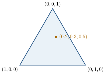
| Notation | x\sim\operatorname{Mult}(n,p) |
| Parameters | n\in\mathbb{Z}^{+}, p\in[0,1]^{K} with \sum_{k=1}^{K}p_k=1 |
| Support | x_k\in\{0,1,\ldots,n\}, \sum_k x_k=n |
| Mass function | p(x)=\frac{n!}{x_1!\cdots x_K!}p_1^{x_1}\cdots p_K^{x_K} |
| Mean | \mathbb{E}(x)=np |
| Variance | \operatorname{Var}(x_k)=np_k(1-p_k) |
| Conjugate prior | Dirichlet distribution: {\boldsymbol{p}}\sim\operatorname{Dirichlet}({\boldsymbol{\alpha}}), giving {\boldsymbol{p}}\mid{\boldsymbol{x}}\sim\operatorname{Dirichlet}({\boldsymbol{\alpha}}+{\boldsymbol{x}}) |
| Listed on | Distribution sheet |
| Properties | 2 |
| Worked examples | 3 |
From the distribution sheet; mode and conjugate pairs from the formula lookup.
The multinomial distribution: parameters, support, probability function, mean and variance.
Properties
Multinomial central limit theorem
Main article: Multinomial central limit theorem
Let {\boldsymbol{x}}\sim\operatorname{Multinomial}(n,{\boldsymbol{p}}) and \widehat{\boldsymbol{p}}={\boldsymbol{x}}/n. For fixed interior {\boldsymbol{p}}, define the covariance matrix
{\color{blue}\boldsymbol{\Sigma}}({\boldsymbol{p}}) =\operatorname{diag}({\boldsymbol{p}})-{\boldsymbol{p}}{\boldsymbol{p}}^{\mathsf T}.
Then
\sqrt n\,(\widehat{\boldsymbol{p}}-{\boldsymbol{p}}) \xrightarrow{\mathcal D} \operatorname{N}_K\!\left( {\boldsymbol{0}}, {\color{blue}\boldsymbol{\Sigma}}({\boldsymbol{p}}) \right).
The covariance matrix is singular because the components of \widehat{\boldsymbol{p}}-{\boldsymbol{p}} sum to zero. On the (K-1)-dimensional simplex, the count cloud therefore tightens at the usual n^{-1/2} rate and becomes locally normal.
Dirichlet–Multinomial conjugacy
Main article: Dirichlet–Multinomial conjugacy
After division by this evidence, \boxed{ {\boldsymbol{p}}\mid{\boldsymbol{x}} \sim\operatorname{Dirichlet}(\alpha_1+x_1,\ldots,\alpha_K+x_K)}.
Examples
Army recruits by IQ class
Worked example from Chi-squared tests
Suppose recruits’ IQ scores are \operatorname{N}(100,16^2), and recruits are classed as 1 (IQ at most 90), 2 (between 90 and 110) or 3 (above 110).
Question. Of 7 new recruits, what is the probability that 2 are in class 1, 4 in class 2 and 1 in class 3?
Solution. The class probabilities are p_1=\Phi\{(90-100)/16\}=\Phi(-0.625)=0.266, p_3=0.266 by symmetry, and p_2=0.468. The class counts are \operatorname{Multinomial}(7;\,0.266,0.468,0.266), so
\mathbb{P}(X_1=2,X_2=4,X_3=1)=\frac{7!}{2!\,4!\,1!}\,0.266^2\times0.468^4\times0.266=0.095.
Q22. Advertising responses and Dirichlet inference
Question page: Q22. Advertising responses and Dirichlet inference
[10 marks]
An advertising campaign records responses from 60 independently sampled people:
| Negative | Neutral | Positive | |
|---|---|---|---|
| Male | 8 | 6 | 16 |
| Female | 12 | 4 | 14 |
Let \mathbf p=(p_{MN},p_{MU},p_{MP},p_{FN},p_{FU},p_{FP}) be the six population cell probabilities, with U denoting a neutral response. Model the counts as multinomial and use \mathbf p\sim\operatorname{Dirichlet}(1,1,1,1,1,1). You may use the Dirichlet kernel f(\mathbf p)\propto\prod_{k=1}^{K}p_k^{\alpha_k-1}, \qquad p_k>0,\quad \sum_{k=1}^{K}p_k=1.
(a) [2 marks] Derive the posterior distribution of \mathbf p, stating its parameters and support.
(b) [2 marks] Find the posterior mean of p_{MP} and its component of the joint MAP estimate of \mathbf p. Explain why that MAP component equals the observed cell proportion here.
(c) [2 marks] Find the posterior predictive probability that one new person responds positively, regardless of gender. Express it as a posterior expectation before calculating it.
(d) [2 marks] For that new person, calculate \mathbb{P}(\text{positive response}\mid\text{female},\text{data}). Explain why this differs from \mathbb{P}(\text{female and positive response}\mid\text{data}).
(e) [2 marks] Are the six components of \mathbf p independent under the posterior? Explain using their constraint.
Definitions. Let D be the observed table and \mathbf p its six population cell probabilities. The labels M,F denote male and female; N,U,P denote negative, neutral, and positive. With parameters a_1,\ldots,a_K>0, a Dirichlet density has kernel \prod_k p_k^{a_k-1} on the simplex p_k>0, \sum_kp_k=1. The joint MAP maximises this density over the entire simplex, not a one-component marginal density.
(a) Posterior distribution. Write the counts in the stated order as \mathbf x=(8,6,16,12,4,14),\qquad n=60. The multinomial likelihood is L(\mathbf p;D)=\frac{60!}{\prod_{k=1}^{6}x_k!} \prod_{k=1}^{6}p_k^{x_k} \propto\prod_{k=1}^{6}p_k^{x_k}. The Dirichlet prior has kernel \prod_k p_k^{1-1}=1 on the simplex. Consequently, p(\mathbf p\mid D)\propto \prod_{k=1}^{6}p_k^{x_k+1-1}, which is the Dirichlet kernel with parameters x_k+1. Thus \boxed{\mathbf p\mid D\sim\operatorname{Dirichlet}(9,7,17,13,5,15).} Its density is supported on the simplex p_k>0, \sum_{k=1}^6p_k=1; the boundary has probability zero. The posterior concentration is A=9+7+17+13+5+15=66.
(b) Posterior mean and MAP. For a Dirichlet vector with parameters a_1,\ldots,a_K and A=\sum_k a_k, \mathbb{E}(p_k)=\frac{a_k}{A},\qquad \widehat p_{k,\mathrm{MAP}}=\frac{a_k-1}{A-K} \quad\text{when every }a_k>1. Here every posterior parameter exceeds one, so \boxed{\mathbb{E}(p_{MP}\mid D)=\frac{17}{66}\approx0.2576,} \qquad \boxed{\widehat p_{MP,\mathrm{MAP}}= \frac{17-1}{66-6}=\frac{16}{60}\approx0.2667.} The MAP component is taken from the mode of the joint posterior for \mathbf p. Since the prior density is constant on the simplex, maximising the posterior is equivalent to maximising the likelihood, giving the observed cell proportions.
(c) Predicting a positive response. Conditional on \mathbf p, the probability of a positive response is p_{MP}+p_{FP}. Averaging over posterior uncertainty gives \begin{aligned} \mathbb{P}(\text{positive}\mid D) &=\int (p_{MP}+p_{FP})p(\mathbf p\mid D)\,d\mathbf p\\ &=\mathbb{E}(p_{MP}+p_{FP}\mid D)\\ &=\frac{17}{66}+\frac{15}{66} =\boxed{\frac{16}{33}\approx0.4848.} \end{aligned} Prediction uses posterior averaging, not substitution of the MAP estimate.
(d) Conditioning on the new person being female. First calculate the two relevant posterior predictive probabilities: \mathbb{P}(\text{female and positive}\mid D)=\mathbb{E}(p_{FP}\mid D)=\frac{15}{66}, \mathbb{P}(\text{female}\mid D) =\mathbb{E}(p_{FN}+p_{FU}+p_{FP}\mid D) =\frac{13+5+15}{66}=\frac{33}{66}. By the definition of conditional probability, \boxed{ \mathbb{P}(\text{positive}\mid\text{female},D) =\frac{15/66}{33/66}=\frac5{11}\approx0.4545. } By contrast, the joint probability is \boxed{\mathbb{P}(\text{female and positive}\mid D) =\frac{15}{66}=\frac5{22}\approx0.2273.} The conditional probability restricts attention to the female row; the joint probability refers to both events occurring for a person sampled from the whole population.
(e) Posterior dependence. No. The probabilities must satisfy \sum_k p_k=1 exactly. Increasing one component leaves less total probability for the others. More formally, if they were independent, then 0=\operatorname{Var}\!\left(\sum_{k=1}^{6}p_k\,\middle|\,D\right) =\sum_{k=1}^{6}\operatorname{Var}(p_k\mid D)>0, a contradiction, since each component has positive posterior variance. Indeed, distinct Dirichlet components have \operatorname{Cov}(p_j,p_k\mid D) =-\frac{a_ja_k}{A^2(A+1)}<0,\qquad j\ne k.
Key result. Add counts to the Dirichlet parameters; average probabilities for prediction; and distinguish a joint cell probability from a probability conditional on a row.
Restaurant ordering methods
Question page: Restaurant ordering methods
A restaurant observed the following numbers of orders yesterday:
| Dine-in | Take-away | Pick-up | Delivery | |
|---|---|---|---|---|
| Count | 63 | 19 | 3 | 38 |
Let {\boldsymbol{p}}=(p_1,p_2,p_3,p_4) be the corresponding population proportions.
With {\boldsymbol{x}}\mid{\boldsymbol{p}}\sim\operatorname{Multinomial}(123,{\boldsymbol{p}}) and {\boldsymbol{p}}\sim\operatorname{Dirichlet}(\alpha_1,\ldots,\alpha_4), identify the posterior.
Last week’s percentages were 44.79\%, 27.60\%, 7.36\%, and 20.25\%. Explain how to use these proportions to choose the direction of {\boldsymbol{\alpha}}, and how a chosen total concentration records the weight given to last week.
Using a prior equivalent, for posterior-mean purposes, to last week’s proportions plus one baseline count in each category, report posterior means and equal-tailed 95\% credible intervals for p_1, p_4, p_1+p_2+p_3, and p_1-p_4.
Question. A restaurant observed the following numbers of orders yesterday:
| Dine-in | Take-away | Pick-up | Delivery | |
|---|---|---|---|---|
| Count | 63 | 19 | 3 | 38 |
Let {\boldsymbol{p}}=(p_1,p_2,p_3,p_4) be the corresponding population proportions.
With {\boldsymbol{x}}\mid{\boldsymbol{p}}\sim\operatorname{Multinomial}(123,{\boldsymbol{p}}) and {\boldsymbol{p}}\sim\operatorname{Dirichlet}(\alpha_1,\ldots,\alpha_4), identify the posterior.
Last week’s percentages were 44.79\%, 27.60\%, 7.36\%, and 20.25\%. Explain how to use these proportions to choose the direction of {\boldsymbol{\alpha}}, and how a chosen total concentration records the weight given to last week.
Using a prior equivalent, for posterior-mean purposes, to last week’s proportions plus one baseline count in each category, report posterior means and equal-tailed 95\% credible intervals for p_1, p_4, p_1+p_2+p_3, and p_1-p_4.
Solution.
The Dirichlet–Multinomial update adds the observed cell counts to the corresponding concentration parameters. Since 63+19+3+38=123, \begin{align*} {\boldsymbol{p}}&\sim\operatorname{Dirichlet}(\alpha_1,\alpha_2,\alpha_3,\alpha_4),\\ {\boldsymbol{x}}\mid{\boldsymbol{p}}&\sim\operatorname{Multinomial}(123,{\boldsymbol{p}}),\\ &\boxed{{\boldsymbol{p}}\mid{\boldsymbol{x}} \sim\operatorname{Dirichlet}(63+\alpha_1,19+\alpha_2,3+\alpha_3,38+\alpha_4)}. \end{align*}
Write last week’s proportions as
{\boldsymbol{q}}=(0.4479,0.2760,0.0736,0.2025).
A Dirichlet prior centred exactly at {\boldsymbol{q}} can be written {\boldsymbol{\alpha}}=\kappa{\boldsymbol{q}}, where \kappa>0 is the total prior concentration. Increasing \kappa preserves the prior mean but increases the weight assigned to last week.
The construction used here instead combines 100 fractional counts with one baseline count in each category:
{\boldsymbol{\alpha}} =(44.79,27.60,7.36,20.25)+(1,1,1,1) =(45.79,28.60,8.36,21.25).
Its concentration is 104 and its mean is {\boldsymbol{\alpha}}/104, which is slightly closer to (1/4,1/4,1/4,1/4) than {\boldsymbol{q}}. Thus the direction and concentration should both be reported; percentages alone determine only the direction.
- The posterior parameters are \begin{align*} {\boldsymbol{\alpha}}^\ast &=(63,19,3,38)+(45.79,28.60,8.36,21.25)\\ &=\boxed{(108.79,47.60,11.36,59.25)}, \end{align*} with total concentration \alpha_0^\ast=108.79+47.60+11.36+59.25=227. Thus
\mathbb{E}(P_1\mid{\boldsymbol{x}})=\frac{108.79}{227}=0.4793, \qquad \mathbb{E}(P_4\mid{\boldsymbol{x}})=\frac{59.25}{227}=0.2610.
Also,
\mathbb{E}(P_1+P_2+P_3\mid{\boldsymbol{x}})=1-\mathbb{E}(P_4\mid{\boldsymbol{x}})=0.7390
and
\mathbb{E}(P_1-P_4\mid{\boldsymbol{x}}) =\frac{108.79-59.25}{227}=0.2182.
The Dirichlet marginal results give \begin{align*} P_1\mid{\boldsymbol{x}}&\sim\operatorname{Beta}(108.79,118.21),\\ P_4\mid{\boldsymbol{x}}&\sim\operatorname{Beta}(59.25,167.75),\\ P_1+P_2+P_3\mid{\boldsymbol{x}}&\sim\operatorname{Beta}(167.75,59.25). \end{align*} Their intervals can therefore be obtained with Beta quantiles. The difference P_1-P_4 has no such Beta form, so simulation handles all four quantities uniformly:
rdirichlet_base <- function(n, alpha) {
  z <- sapply(alpha, function(a) rgamma(n, shape = a, rate = 1))
  z / rowSums(z)
}

set.seed(3500)
alpha_post <- c(108.79, 47.60, 11.36, 59.25)
p <- rdirichlet_base(100000, alpha_post)
summaries <- cbind(
  p1 = p[, 1],
  p4 = p[, 4],
  p123 = rowSums(p[, 1:3]),
  difference = p[, 1] - p[, 4]
)
rbind(
  mean = colMeans(summaries),
  lower = apply(summaries, 2, quantile, 0.025),
  upper = apply(summaries, 2, quantile, 0.975)
)
For the displayed seed, rounding to three decimals gives
| Quantity | Posterior mean | 2.5% | 97.5% |
|---|---|---|---|
| p_1 | 0.479 | 0.415 | 0.544 |
| p_4 | 0.261 | 0.206 | 0.320 |
| p_1+p_2+p_3 | 0.739 | 0.680 | 0.794 |
| p_1-p_4 | 0.218 | 0.109 | 0.325 |
The first three intervals agree, apart from Monte Carlo rounding, with the corresponding exact Beta quantiles.
Used in
- Listed on the distribution sheet.
- Also used in Joint distributions · Categorical data and the Dirichlet distribution