The Beta–Binomial model
Part of Bayesian statistics · 11 questions on this topic · What links here
The Beta–Binomial model
| Part | Bayesian statistics |
| Chapter | 2 of 9 in this part |
| Previous | Bayesian foundations |
| Next | Conjugate analysis for normal models |
| Questions | 11 |
| Definitions | Beta distribution |
| Results | Beta–Binomial conjugacy · Sequential coherence · Beta–Binomial posterior prediction |
| Figures | 1 |
Coin tossing and the likelihood
Let Y_i=1 denote a head on toss i and Y_i=0 a tail. Conditional on the unknown probability \theta,
Y_i\mid\theta\stackrel{\mathrm{iid}}{\sim}\operatorname{Bern}(\theta), \qquad 0\leq\theta\leq1.
For an observed sequence y_1,\ldots,y_n with x=\sum_{i=1}^ny_i heads, \begin{align*} p(y_1,\ldots,y_n\mid\theta) &=\prod_{i=1}^n\theta^{y_i}(1-\theta)^{1-y_i}\\ &=\theta^{\sum_i y_i}(1-\theta)^{\sum_i(1-y_i)}\\ &=\theta^x(1-\theta)^{n-x}. \end{align*} If only the count X=\sum_iY_i is observed, then all \binom{n}{x} sequences with x heads are collected together: p(x\mid\theta)=\binom{n}{x}\theta^x(1-\theta)^{n-x}. \qquad(1) The combinatorial term matters for probabilities of X, but it is constant in \theta and can be removed from the likelihood kernel.
The Beta prior
Definition 1 (Beta distribution) For \alpha,\beta>0, the Beta density is p(\theta\mid\alpha,\beta) =\frac{1}{B(\alpha,\beta)} \theta^{\alpha-1}(1-\theta)^{\beta-1}, \qquad 0<\theta<1, \qquad(2) where
B(\alpha,\beta) =\int_0^1t^{\alpha-1}(1-t)^{\beta-1}\,\mathrm{d} t =\frac{\Gamma(\alpha)\Gamma(\beta)} {\Gamma(\alpha+\beta)}.
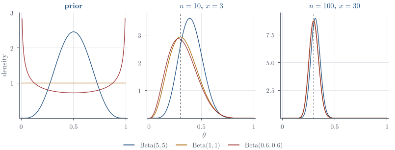
Three symmetric priors make the contrast concrete:
\operatorname{Beta}(5,5), concentrated around 1/2;
\operatorname{Beta}(1,1), uniform on [0,1]; and
\operatorname{Beta}(0.6,0.6), with greater density near 0 and 1.
For an ordinary circulating coin, \operatorname{Beta}(5,5) is the most defensible of these three: manufacturing makes values near 1/2 more plausible than values near 0 or 1, while symmetry does not favour heads over tails. If the experiment itself supplies no preferred face, that symmetry is the stable description. A uniform prior assigns equal mass to every interval of the same width, including physically extreme intervals near the endpoints. The U-shaped prior instead represents suspicion that the coin is strongly biased, not ignorance in a neutral sense.
There is no context-free “correct prior for a coin.” The population of coins matters. A newly minted circulating coin, a stage magician’s coin, and a coin selected because it behaved strangely are different prior problems. Calling a prior neutral does not make it so: even the uniform prior gives substantial weight to physically extreme biases. The defensible choice is the one whose implications match how the object entered the experiment.
Persi Diaconis made the same contextual point with a mechanical coin-flipping machine: what looks random at one level may be largely determined once the initial conditions are controlled.1
Rare data remain possible. Under a fair coin, ten heads in ten tosses has probability 2^{-10}=1/1024; it is surprising, not logically impossible. For \alpha,\beta>1,
\mathbb{E}(\theta)=\frac{\alpha}{\alpha+\beta}, \qquad \operatorname{mode}(\theta) =\frac{\alpha-1}{\alpha+\beta-2},
and for all \alpha,\beta>0,
\operatorname{Var}(\theta) =\frac{\alpha\beta} {(\alpha+\beta)^2(\alpha+\beta+1)}.
Conjugate update with every constant shown
Multiplying Equation 1 and Equation 2 gives \begin{align*} p(x\mid\theta)p(\theta) &=\binom{n}{x}\theta^x(1-\theta)^{n-x} \frac{\theta^{\alpha-1}(1-\theta)^{\beta-1}} {B(\alpha,\beta)}\\ &=\frac{\binom{n}{x}}{B(\alpha,\beta)} \theta^{x+\alpha-1} (1-\theta)^{n-x+\beta-1}. \end{align*} The integral of the last two factors is B(x+\alpha,n-x+\beta), so the evidence is \begin{aligned} p(x) &=\int_0^1p(x\mid\theta)p(\theta)\,\mathrm{d}\theta\\ &=\binom{n}{x} \frac{B(x+\alpha,n-x+\beta)}{B(\alpha,\beta)}. \end{aligned} \qquad(3) Dividing by this evidence cancels the binomial coefficient and the old Beta constant: \begin{align*} p(\theta\mid x) &=\frac{p(x\mid\theta)p(\theta)}{p(x)}\\ &=\frac{ \theta^{x+\alpha-1}(1-\theta)^{n-x+\beta-1}} {B(x+\alpha,n-x+\beta)}. \end{align*}
Proposition 1 (Beta–Binomial conjugacy) Therefore \boxed{ \theta\mid x\sim \operatorname{Beta}(\alpha+x,\beta+n-x)}. \qquad(4)
The update is “prior successes plus observed successes” and “prior failures plus observed failures.” The Beta family is conjugate to the binomial likelihood because the posterior is another Beta density.
Worked prior-sensitivity calculation
For n=10 tosses and x=3 heads, these three priors give \begin{align*} \operatorname{Beta}(5,5)&\longrightarrow\operatorname{Beta}(8,12),\\ \operatorname{Beta}(1,1)&\longrightarrow\operatorname{Beta}(4,8),\\ \operatorname{Beta}(0.6,0.6)&\longrightarrow\operatorname{Beta}(3.6,7.6). \end{align*} For example, under the uniform prior,
\mathbb{E}(\theta\mid x)=\frac4{12}=\frac13, \qquad \widehat\theta_{\mathrm{MAP}} =\frac{4-1}{4+8-2}=\frac3{10}=0.3.
The posterior probability of downward bias is
\mathbb{P}(\theta<0.5\mid x) =\int_0^{0.5}\frac{\theta^3(1-\theta)^7}{B(4,8)}\,\mathrm{d}\theta.
With n=100 and x=30 heads, the same priors give \begin{align*} \operatorname{Beta}(5,5)&\longrightarrow\operatorname{Beta}(35,75),\\ \operatorname{Beta}(1,1)&\longrightarrow\operatorname{Beta}(31,71),\\ \operatorname{Beta}(0.6,0.6)&\longrightarrow\operatorname{Beta}(30.6,70.6). \end{align*} The relative effect of the prior is smaller because the data contribute 100 counts while the first prior contributes a fixed amount.
Direct substitution of x=30 in Equation 4 gives the first shape parameters 35, 31, and 30.6 written above. The values 36, 32, and 31.6 are one unit larger and do not follow from that substitution. The second shape parameters that match x=30 are 75, 71, and 70.6.
Pseudo-counts and sequential updating
The posterior mean is \begin{align*} \mathbb{E}(\theta\mid x) &=\frac{x+\alpha}{n+\alpha+\beta}\\ &=\frac{n}{n+\alpha+\beta}\frac{x}{n} +\frac{\alpha+\beta}{n+\alpha+\beta} \frac{\alpha}{\alpha+\beta}. \end{align*} Thus \alpha+\beta acts as a prior sample size for the posterior mean, with \alpha prior heads and \beta prior tails.
For the posterior mode, \begin{align*} \widehat\theta_{\mathrm{MAP}} &=\frac{x+\alpha-1}{n+\alpha+\beta-2}\\ &=\frac{n}{n+\alpha+\beta-2}\frac{x}{n} +\frac{\alpha+\beta-2}{n+\alpha+\beta-2} \frac{\alpha-1}{\alpha+\beta-2}, \end{align*} provided the updated parameters exceed one. Hence \alpha-1 and \beta-1 are the natural pseudo-counts for mode calculations. The two conventions do not contradict each other; they correspond to different posterior summaries.
Remark 1 (Two pseudo-count conventions). For posterior means, (\alpha,\beta) act as prior success and failure counts. For an interior posterior mode, the corresponding counts are (\alpha-1,\beta-1). A pseudo-count statement is incomplete unless the posterior summary being interpreted is also named.
Relative to \operatorname{Beta}(1,1), the prior \operatorname{Beta}(5,5) contributes four additional heads and four additional tails in the mode-based convention. That is eight prior trials, not “four heads in four trials.”
Proposition 2 (Sequential coherence) Sequential updating is exact. If data arrive in batches (x_1,n_1) and (x_2,n_2), then \begin{align*} \theta\mid x_1 &\sim\operatorname{Beta}(\alpha+x_1,\beta+n_1-x_1),\\ \theta\mid x_1,x_2 &\sim\operatorname{Beta}(\alpha+x_1+x_2, \beta+n_1+n_2-x_1-x_2), \end{align*} which is the same posterior obtained by combining both batches first.
Nonconjugate priors
Remark 2 (Conjugacy is optional). Conjugacy is convenient, not compulsory. A prior concentrated around 1/2 could be obtained by truncating a Laplace density:
p(\theta)\propto \exp\!\left(-\frac{|\theta-1/2|}{b}\right) \mathbf{1}\{0\leq\theta\leq1\}.
The posterior kernel is then
p(\theta\mid x) \propto \theta^x(1-\theta)^{n-x} \exp\!\left(-\frac{|\theta-1/2|}{b}\right) \mathbf{1}\{0\leq\theta\leq1\}.
If equality rather than proportionality is needed, symmetry supplies the normalising constant without numerical integration: \begin{align*} \int_0^1\exp\!\left(-\frac{|\theta-1/2|}{b}\right)\,\mathrm{d}\theta &=2\int_0^{1/2}\exp\!\left(-\frac{1/2-\theta}{b}\right)\,\mathrm{d}\theta\\ &=2\left[b\exp\!\left(-\frac{1/2-\theta}{b}\right)\right]_{\theta=0}^{1/2}\\ &=2b\left(1-e^{-1/(2b)}\right). \end{align*} Thus the proper truncated-Laplace prior has multiplier ([2b{1-e^{-1/(2b)}}]^{-1}). The resulting posterior is not a named standard density, so its normalising integral and summaries must be evaluated numerically. The later MCMC chapters provide a general route when direct integration becomes difficult.
The difficulty scales with dimension. A one-dimensional posterior can be normalised by quadrature; a direct grid with m points in each of d coordinates requires m^d evaluations. This exponential growth is the computational reason that nonconjugate multiparameter models lead to Monte Carlo methods.
Conjugacy is a computational convenience, not a modelling command. It was especially attractive when integration and simulation were expensive, and it remains valuable because it exposes the update algebra. But if a scientifically sensible prior is nonconjugate, the right response is usually to improve the computation rather than replace the prior merely to obtain a named posterior. Likewise, the MAP can be useful, particularly in optimisation, but one point is not a substitute for the posterior uncertainty that motivated Bayesian analysis in the first place.
Beta–Binomial prediction
The prior predictive probability of X=x is already given by Equation 3. Expanding the Beta functions gives the Beta–Binomial mass function:
p(x) =\binom{n}{x} \frac{\Gamma(x+\alpha)\Gamma(n-x+\beta)} {\Gamma(n+\alpha+\beta)} \frac{\Gamma(\alpha+\beta)} {\Gamma(\alpha)\Gamma(\beta)}.
For one future toss \widetilde Y, conditional independence gives \begin{align*} \mathbb{P}(\widetilde Y=1\mid x) &=\int_0^1\mathbb{P}(\widetilde Y=1\mid\theta) p(\theta\mid x)\,\mathrm{d}\theta\\ &=\int_0^1\theta p(\theta\mid x)\,\mathrm{d}\theta\\ &=\mathbb{E}(\theta\mid x)\\ &=\frac{x+\alpha}{n+\alpha+\beta}. \end{align*} For m future tosses and \widetilde X future heads, \begin{align*} p(\widetilde x\mid x) &=\int_0^1 \binom{m}{\widetilde x} \theta^{\widetilde x}(1-\theta)^{m-\widetilde x} \frac{\theta^{x+\alpha-1} (1-\theta)^{n-x+\beta-1}} {B(x+\alpha,n-x+\beta)}\,\mathrm{d}\theta\\ &=\binom{m}{\widetilde x} \frac{B(\widetilde x+x+\alpha, m-\widetilde x+n-x+\beta)} {B(x+\alpha,n-x+\beta)}. \end{align*} This is a Beta–Binomial posterior predictive distribution.
Proposition 3 (Beta–Binomial posterior prediction) If \theta\mid x\sim\operatorname{Beta}(a,b) and, conditionally on \theta, \widetilde X\sim\operatorname{Bin}(m,\theta), then
\mathbb{P}(\widetilde X=k\mid x) =\binom mk\frac{B(k+a,m-k+b)}{B(a,b)}, \qquad k=0,\ldots,m.
For one future Bernoulli observation, \mathbb{P}(\widetilde Y=1\mid x)=a/(a+b).
Numerical example: five future tosses
Example 1 (Five future tosses) Suppose the prior is \theta\sim\operatorname{Beta}(2,2) and the observed data contain x=8 heads in n=10 tosses.
Question. Find the posterior predictive probability of a head on the next toss and the probability of at least four heads in five future tosses. Derive the predictive variance for the five-toss count and compare it with the variance obtained by plugging the posterior mean of \theta into a Binomial model.
Solution. The posterior calculation gives
\theta\mid x \sim\operatorname{Beta}(2+8,2+10-8) =\operatorname{Beta}(10,4).
For the very next toss, \begin{align*} \mathbb{P}(\widetilde Y=1\mid x) &=\mathbb{E}(\theta\mid x)\\ &=\frac{10}{10+4}\\ &=\frac57\\ &\approx0.714. \end{align*} The raw sample proportion is 8/10=0.8. The prediction is less extreme because it averages over the posterior produced by the data and the \operatorname{Beta}(2,2) prior.
Now let \widetilde X be the number of heads in m=5 future tosses. With a=10, b=4, and T=a+b=14, \mathbb{P}(\widetilde X=k\mid x) =\binom5k\frac{B(k+a,5-k+b)}{B(a,b)}, \qquad k=0,\ldots,5. \qquad(5) For the rising factorial
(c)^{\overline r} =c(c+1)\cdots(c+r-1), \qquad (c)^{\overline 0}=1,
the Beta-function ratio satisfies
\frac{B(k+a,5-k+b)}{B(a,b)} =\frac{(a)^{\overline k}(b)^{\overline{5-k}}} {(a+b)^{\overline5}}.
Therefore the probability of at least four heads is \begin{align*} \mathbb{P}(\widetilde X\geq4\mid x) &=\mathbb{P}(\widetilde X=4\mid x) +\mathbb{P}(\widetilde X=5\mid x)\\ &=\frac{ \binom54(10)^{\overline4}(4)^{\overline1} +\binom55(10)^{\overline5}(4)^{\overline0}} {(14)^{\overline5}}\\ &=\frac{ 5(10\cdot11\cdot12\cdot13)(4) +(10\cdot11\cdot12\cdot13\cdot14)} {14\cdot15\cdot16\cdot17\cdot18}\\ &=\frac{583440}{1028160}\\ &\approx0.567. \end{align*}
This example also shows exactly why posterior prediction is more dispersed than a plug-in Binomial distribution. Conditional on \theta,
\mathbb{E}(\widetilde X\mid\theta)=5\theta, \qquad \operatorname{Var}(\widetilde X\mid\theta)=5\theta(1-\theta).
For \theta\mid x\sim\operatorname{Beta}(a,b) with T=a+b,
\mathbb{E}(\theta\mid x)=\frac aT, \qquad \operatorname{Var}(\theta\mid x)=\frac{ab}{T^2(T+1)}.
Moreover, \begin{align*} \mathbb{E}\{\theta(1-\theta)\mid x\} &=\mathbb{E}(\theta\mid x)-\mathbb{E}(\theta^2\mid x)\\ &=\frac aT-\frac{a(a+1)}{T(T+1)}\\ &=\frac{a(T+1)-a(a+1)}{T(T+1)}\\ &=\frac{a(T-a)}{T(T+1)}\\ &=\frac{ab}{T(T+1)}. \end{align*} Applying Equation (3) in Bayesian foundations, \begin{align*} \operatorname{Var}(\widetilde X\mid x) &=\mathbb{E}\{5\theta(1-\theta)\mid x\} +\operatorname{Var}(5\theta\mid x)\\ &=\frac{5ab}{T(T+1)} +\frac{25ab}{T^2(T+1)}\\ &=\frac{5ab(T+5)}{T^2(T+1)}\\ &=\frac{5(10)(4)(19)}{14^2(15)}\\ &=\frac{190}{147}\\ &\approx1.293. \end{align*} If one instead plugs in the posterior mean \widehat\theta=10/14, the variance would be only
5\widehat\theta(1-\widehat\theta) =5\left(\frac{10}{14}\right)\left(\frac4{14}\right) =\frac{50}{49} \approx1.020.
The difference is the second term in Equation (3) in Bayesian foundations: uncertainty about \theta.
Questions on this topic
Open a question to attempt it. Its worked answer is folded away at the bottom of the page.
What links here
Pages (4)
- Categorical data and the Dirichlet distribution — via pseudo-count
- Exponential families and conjugacy — via Beta–Binomial
- Hierarchical Bayes — via Beta distribution
- Reference formulas and problem-solving workflow — via pseudo-count
Questions and answers (8)
- A future run of tosses · A geometric observation and a uniform prior · Q6 (answer) · Q17 (answer) · Q23 · Q44 (answer) · Question 11 (answer) · Question 14 (answer)
See also
Footnotes
Persi Diaconis, who worked as a magician before becoming a mathematician and statistician at Stanford, is the source of this mechanical coin-flipping discussion; see the Stanford Mathematics profile.↩︎