Random slopes, and a binary mixed model
Part of Correlated data · 6 questions on this topic · What links here
Random slopes, and a binary mixed model
| Part | Correlated data |
| Chapter | 2 of 4 in this part |
| Previous | Random intercepts |
| Next | Marginal models, and two responses at once |
| Questions | 6 |
| Figures | 2 |
A shared intercept is the smallest mixed model. Blocks can also change slopes. This chapter fits that model to a sleep-deprivation study, and then replaces the normal residual by a Bernoulli likelihood for a contraception survey.
A slope that belongs to the block
Write {\boldsymbol{Z}}_{ji} for the covariates whose effects are allowed to vary by block. They may be the same as {\boldsymbol{X}}_{ji}, or a subset, or something else. Y_{ji} ={\boldsymbol{X}}_{ji}^\top\boldsymbol{\beta} +{\boldsymbol{Z}}_{ji}^\top\boldsymbol{\alpha}_j +\varepsilon_{ji}, \boldsymbol{\alpha}_j\stackrel{\mathrm{ind}}{\sim}\mathrm{N}({\boldsymbol{0}},{\color{blue}\boldsymbol{\Sigma}}_A), \qquad \varepsilon_{ji}\stackrel{\mathrm{ind}}{\sim}\mathrm{N}(0,\sigma^2). {\color{blue}\boldsymbol{\Sigma}}_A holds the variances of the random intercept and the random slopes, and the covariances between them. Dropping every random slope returns the model of the previous chapter. We start from the larger model when a covariate might interact with the block: some hospitals are better at some treatments, some drivers deteriorate faster when they are not allowed to sleep.
A fixed effect is a constant. Repeat the experiment and it is the same constant. A random effect is a draw. Repeat the sleep study and eighteen different drivers are drawn, and the eighteen intercepts and slopes are new. We estimate the mean and the covariance of that population. Predicting the eighteen draws we happened to get is a different task, and it is a prediction of a random variable, not an estimate of a fixed parameter. With the variances known, that prediction is the best linear unbiased predictor. With the variances estimated, it is the empirical version of the same thing. Software computes it. We do not derive it by hand.
Sleep deprivation
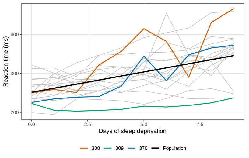
Eighteen subjects, treated as a sample of long-distance drivers rather than as eighteen named people, were restricted to three hours of sleep a night for ten days. Each day their reaction time was an average of several ruler-drop trials, in milliseconds. Most people slow down. One or two stay flat, and one seems to get slightly faster, which is the pattern if three hours was more sleep than they usually had. Before looking, the reasonable model is a person-specific intercept and a person-specific slope on day. Reflexes differ, and so does the damage from another night of three hours.
need <- function(pkg) {
  if (!requireNamespace(pkg, quietly = TRUE)) {
    install.packages(pkg, repos = "https://cloud.r-project.org")
  }
  suppressPackageStartupMessages(library(pkg, character.only = TRUE))
}
need("lme4")
data(sleepstudy, package = "lme4")
fit <- lmer(Reaction ~ Days + (Days | Subject), data = sleepstudy)
summary(fit)
fit0 <- lmer(Reaction ~ Days + (1 | Subject), data = sleepstudy)
anova(fit0, fit)
round(ranef(fit)$Subject[c("308", "309", "370"), ], 1)
The (Days | Subject) term is a random intercept and a random slope on day, with a correlation between them. The fit is by restricted maximum likelihood. The estimates are
Random effects:
 Subject  (Intercept)   variance 612.09    sd 24.74
          Days          variance  35.07    sd  5.92    corr 0.07
 Residual               variance 654.94    sd 25.59

Fixed effects:
 (Intercept)   251.41     se 6.83
 Days           10.47     se 1.55
These are statements about the population the eighteen were drawn from, not about the eighteen. The average driver starts at 251 milliseconds and slows by 10.5 milliseconds per day of deprivation. A typical driver sits 25 milliseconds away from that starting value, and a typical slope sits 5.9 milliseconds per day away from 10.5. The correlation between a driver’s intercept and slope is 0.07. Someone who is slow on day zero is not, in any important way, someone who deteriorates faster.
Whether the random slopes are needed is a comparison of this fit with Reaction ~ Days + (1 | Subject). The likelihood-ratio statistic is 42.1 on 2 degrees of freedom, and the printed p-value is 7\times 10^{-10}. That p-value is not an exact chi-squared tail probability. The null hypothesis puts a variance on the boundary of the parameter space, at zero, so the usual asymptotic distribution does not apply. The printed tail probability is conservative: it is larger than the p-value from the correct mixture of chi-squared laws. A conservative p-value this small is still small. The slopes stay. Had the printed value been 0.07, it would not be clear which side of 0.05 the proper test sat on, and the term would not be dropped on the strength of the printed value.
The empirical predictors of the eighteen deviations are a different object again. Subject 308 is predicted about 2 milliseconds slower than the population intercept and about 9 milliseconds per day steeper than the population slope. Subject 309 is about 40 milliseconds faster at the start and has a slope about 8 below the average, which is why that series looks flat: 10.5-8 is nearly zero. Subject 370 starts faster than average and then falls away faster than average.
Repeat the study and none of these eighteen numbers returns. The fixed effects 251 and 10.5 are the quantities that are supposed to.
A Bernoulli response
The outer distribution does not have to be normal. Keep the linear predictor, random intercept and random slopes included, and let Y_{ji}\mid {\boldsymbol{X}}_{ji},\boldsymbol{\alpha}_j \stackrel{\mathrm{ind}}{\sim} \mathrm{Bernoulli}\!\left( \mu\bigl({\boldsymbol{X}}_{ji}^\top\boldsymbol{\beta}+{\boldsymbol{Z}}_{ji}^\top\boldsymbol{\alpha}_j\bigr) \right), with \boldsymbol{\alpha}_j still multivariate normal on the link scale. For a logit, \mu is the expit. The normal distribution on \boldsymbol{\alpha}_j is a modelling choice about a latent intercept, not a claim that we observed a normal measurement. It is a distribution we can interpret, and there is no stronger reason, before seeing the data, to pick a different one. The likelihood integrates the random effects out. There is no closed form, and no single algorithm that is guaranteed to find the maximum in every data set. When the numerical answer is in doubt, we fit the model more than one way, and we trust an agreement.
The 1989 Bangladesh fertility survey has 1934 women and a binary response: currently using contraception, or not. Age is centred and enters as a quadratic, because use should rise and then fall rather than climb forever. ch records whether she already has a living child. urban records urban against rural. district is the cluster. Women in the same district share facilities and customs, so a district intercept is the natural random effect. If every district in the country were in the sample, “a draw from a population of districts” would be a fiction about the boundaries of districts rather than about a sampling frame. We still use it. The districts that exist are one way of cutting the map.
need <- function(pkg) {
  if (!requireNamespace(pkg, quietly = TRUE)) {
    install.packages(pkg, repos = "https://cloud.r-project.org")
  }
  suppressPackageStartupMessages(library(pkg, character.only = TRUE))
}
need("lme4")
need("mlmRev")
data(Contraception, package = "mlmRev")
# age is already centred in this copy of the survey
Contraception$ch <- as.integer(Contraception$livch != "0")
Contraception$age2 <- Contraception$age^2
# a warning about rescaling age and age2 can appear; the estimates are the table below
summary(glmer(use ~ age + age2 + urban + ch + (1 | district),
              data = Contraception, family = binomial))
There are 60 districts. The district intercept has estimated standard deviation 0.474 on the log-odds scale: from district to district, at a fixed age, urban status, and child status, the log-odds of use move by about half a unit. The fixed effects are
(Intercept)  -1.006    se 0.169    z -5.95
age           0.0063   se 0.0079   z  0.79
age2         -0.00464  se 0.00072  z -6.43
urbanY        0.693    se 0.121    z  5.74
ch            0.860    se 0.148    z  5.80
Age has a positive linear term that is not itself significant and a negative square that is. Together they are the upside-down parabola.
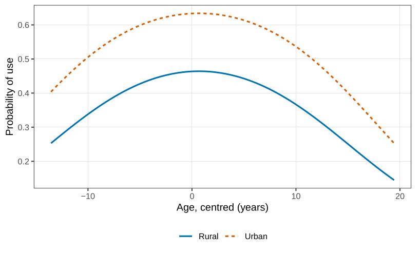
The linear coefficient is not interpreted on its own. Urban women have odds of use \exp(0.693)=2.00 times those of rural women in the same district, at the same age and the same child status. A woman who already has a living child has odds \exp(0.860)=2.36 times those of a woman who does not. The district standard deviation is a typical shift, not a comparison of two named districts.
The urban contrast need not be the same in every district. A large city can have a rural fringe that is not very different from the centre. A small regional centre can have a sharp drop just outside the town. Some districts in the file are entirely urban, so a rural contrast for them is a prediction about a place that is not there.
need <- function(pkg) {
  if (!requireNamespace(pkg, quietly = TRUE)) {
    install.packages(pkg, repos = "https://cloud.r-project.org")
  }
  suppressPackageStartupMessages(library(pkg, character.only = TRUE))
}
need("lme4")
need("mlmRev")
data(Contraception, package = "mlmRev")
Contraception$ch <- as.integer(Contraception$livch != "0")
Contraception$age2 <- Contraception$age^2
summary(glmer(use ~ age + age2 + urban + ch + (urban | district),
              data = Contraception, family = binomial))
The average urban coefficient is now 0.770 (z=4.69): across districts, urban versus rural is a factor of \exp(0.77)\approx 2.16 on the odds. The district-level standard deviation of that contrast is 0.74, almost as large as the average contrast itself. Some districts have essentially no urban gap. Some have a much larger one. The correlation between the district intercept and the district urban slope is -0.79. A district that already has high use has a smaller urban-rural gap. Where use is common, rural and urban are not far apart, and where use is uncommon the town centre and the countryside are. The likelihood-ratio comparison with the random-intercept-only model is small enough, even as a conservative boundary p-value, that the extra random slope stays. It is an interaction. The effect of living in town depends on the district.
Marginal models, which describe the population average without a mechanism for the correlation, are the next chapter.
The sleep-study random-slope variance is 35.07. Convert it to a standard deviation and say what “a typical driver” means for the daily change in reaction time.
Why is the p-value on \sigma^2_{\text{slope}}=0 not a chi-squared tail probability, and in which direction is the printed value wrong?
From the contraception fit with a random intercept only, compute \exp(0.693) and \exp(0.860) and state both as odds ratios with the covariates that are being held fixed.
The correlation between a district’s intercept and its urban slope is -0.79. Give the direction of that statement in one sentence, without using the word “significant”.
Questions on this topic
Open a question to attempt it. Its worked answer is folded away at the bottom of the page.
What links here
Questions and answers (5)
- Q41 (answer) · Question 20 · Question 22 (answer) · C35 · C37