Additive smooths
Part of Smoothing · 2 questions on this topic · What links here
Additive smooths
| Part | Smoothing |
| Chapter | 2 of 2 in this part |
| Previous | Smooth means |
| Questions | 2 |
| Figures | 1 |
A smooth function of one covariate was enough to let kyphosis rise and fall with age. This chapter puts more than one covariate into that smooth.
Sums of smooth functions
A completely free surface g(x_1,x_2,x_3) can be fitted, and in four covariates it cannot even be pictured. We do not use it. The model that stays readable replaces the linear predictor by a sum of univariate smooths, one per covariate. On the logit scale for kyphosis,
\mathrm{logit}\,\mathrm{P}(\text{kyphosis})
=\beta_0+g_1(\text{number})+g_2(\text{start})+g_3(\text{age}).
Each g_j has its own penalty. Nothing forces them to be equally smooth. This is a generalised additive model, in the sense of Hastie and Tibshirani: additive in the smooths, not linear in the covariates. Number takes only the values 1 through 8, and Start only sixteen vertebral positions, so a smooth cannot have more knots than there are distinct values.
need <- function(pkg) {
  if (!requireNamespace(pkg, quietly = TRUE)) {
    install.packages(pkg, repos = "https://cloud.r-project.org")
  }
  suppressPackageStartupMessages(library(pkg, character.only = TRUE))
}
need("mgcv")
need("rpart")
data(kyphosis, package = "rpart")
kyphosis$Kyphosis <- as.numeric(kyphosis$Kyphosis == "present")
summary(gam(Kyphosis ~ s(Number, k = 8) + s(Start, k = 16) + s(Age),
            family = binomial, data = kyphosis))
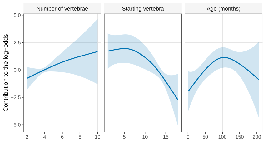
The equivalent degrees of freedom are about 1.19 for the number of vertebrae, 2.04 for the starting position, and 2.21 for age.
In Figure 1, number is almost a straight line on the log-odds scale: more vertebrae in the same operation, higher odds of kyphosis. Start is flat from the top of the spine through about the sixth vertebra and then falls. Surgery that begins low on the back has the smaller risk. Age, now conditional on the other two, still rises and then eases, a little less dramatically than when it was the only covariate.
Each curve is the effect of moving that one covariate while the others are held fixed. Holding the starting vertebra at 16 and imagining ten vertebrae below it is not a spine that exists. The sentence is conditional on a hypothetical, and some of those hypotheticals are empty.
A free function of all three covariates together would fit a surface we could not explain to a surgeon. Two-way interactions are already hard. Three-way interactions are where we stop. The compromise is a partially linear model: a coefficient for the term you want a unit-change sentence about, and a smooth for the terms you are only adjusting for. Ambient temperature in a lab, or the weight of a patient in a trial of two treatments, is the second kind. Dose and treatment are the first kind.
Number of vertebrae looked linear, so force it to be a slope and leave start and age smooth:
need <- function(pkg) {
  if (!requireNamespace(pkg, quietly = TRUE)) {
    install.packages(pkg, repos = "https://cloud.r-project.org")
  }
  suppressPackageStartupMessages(library(pkg, character.only = TRUE))
}
need("mgcv")
need("rpart")
data(kyphosis, package = "rpart")
kyphosis$Kyphosis <- as.numeric(kyphosis$Kyphosis == "present")
summary(gam(Kyphosis ~ Number + s(Start, k = 16) + s(Age),
            family = binomial, data = kyphosis))
The slope on number is 0.333 with standard error 0.232 (z=1.43, p=0.15). Once start and age are in the model, the number of vertebrae is not detected. We would drop it. Start remains, with equivalent degrees of freedom about 2.03. One printout gave p=0.013 for start and p=0.071 for age; mgcv 1.8 prints about 0.015 and 0.078. Age stays borderline either way, and we keep it for the same reason as in the previous chapter. The important covariate is where the operation starts. On the plotted smooth, the log-odds for a start among vertebrae 1 to 5 sit several units above the log-odds for a start at the bottom of the spine. That gap can be read as a factor of about \exp(5)=148 on the odds scale. A gap of 4, which is also a fair reading of the same curve, is \exp(4)\approx 55. We will not pretend the graph yields one integer. The comparison is large, it favours starting lower, and it is conditional on age.
Smooth the covariates you are adjusting for and do not need a one-sentence answer about. Keep a parametric term for the covariate whose unit change you intend to report. A smooth of everything is a picture, not an effect.
- In the additive kyphosis model,
Numberhas equivalent degrees of freedom 1.19. Say what that number claims about the shape on the log-odds scale, and whyk = 8is a ceiling rather than a target.
Questions on this topic
Open a question to attempt it. Its worked answer is folded away at the bottom of the page.
What links here
Pages (1)
- How to use the final preparation — via GAM
Questions and answers (6)
- Q36 (answer) · Q37 (answer) · Q38 (answer) · Question 19 (answer) · Question 21 · C33