Categorical responses

Part of Generalised linear models · 3 questions on this topic · What links here

Categorical responses

Fitted cumulative probabilities against exposure time.

Part	Generalised linear models
Chapter	4 of 6 in this part
Previous	Underdispersion, positive responses, and quasi-likelihood
Next	Paired comparisons, and how far a fit is from the data
Questions	3
Definitions	Proportional-odds model · Baseline-category logit model
Figures	1

A response that can only land in one of K fixed categories is polytomous. There is no mean of the category labels that we are willing to interpret. A grade of 7 is not seven times a grade of 1, and the average of “rugby”, “cricket”, and “netball” is not a sport. What is well defined is the probability of each category.

Three kinds of scale show up in practice.

1. Nominal: the labels are exchangeable. Blood type, a sport preference, a car brand listed alphabetically. Any order you write them down is your order, not the data’s.
2. Ordinal: there is a better and a worse, or a stronger and a milder, and the numbers you attach do nothing except record that order. A Likert item, a pain score, a university grade. Nobody is trying to land on exactly a 6. They are trying to land on a 6 or better.
3. Interval: the rare case in which the categories are bins of a real measurement, such as income brackets, and the midpoint of a bin is a number you could average. Everything else on this list is not that.

Write p_k=\mathrm{P}(Y\text{ is in category }k). For an ordinal scale we would rather work with the upper tail, because “at least this good” is the question people ask: \gamma_k=\mathrm{P}(Y\ge k). The tails determine the category probabilities and the other way around. \gamma_1=1 if category 1 is the bottom of the scale, because everyone is at least in the lowest category. Cumulative probabilities are meaningless if the labels have no order. For a nominal response we stay with the p_k.

“Association” is the word. “Correlation” is for two numerical variables. A grade is not numerical, so hours of study are associated with higher grades. They are not correlated with the grade labels.

Ordinal data, built from binary splits

Food scores, pain scores, and agreement scales have cutpoints that are partly conventional. If we collapse “strongly agree” into “agree”, the form of the model should survive. The estimates will change, because information was thrown away. The equation should be the same kind of equation. That requirement is what forces cumulative probabilities rather than a separate model for each p_k.

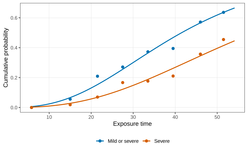
Three categories are enough to see it. In the pneumonia experiment, animals were exposed to a bacterium for a logged time x=\log(\text{exposure in seconds}), and the response was 1 none, 2 mild, 3 severe. Sample size falls as the dose rises, which is the ethical constraint you would hope for. The rows, with x=\log t, are

seconds	x	none	mild	severe
5.8	1.76	98	0	0
15.0	2.71	51	2	1
21.5	3.07	34	6	3
27.5	3.31	35	5	8
33.5	3.51	32	10	9
39.5	3.68	23	7	8
46.0	3.83	12	6	10
51.5	3.94	4	2	5

Suppose the only question is whether any pneumonia occurred. Mild and severe collapse into one category, and the problem is binary: \mathrm{P}(Y\ge 2)=\frac{\exp(\beta_{0,\mathrm{ms}}+\beta_{1,\mathrm{ms}} x)}{1+\exp(\beta_{0,\mathrm{ms}}+\beta_{1,\mathrm{ms}} x)}. Suppose instead that mild disease is treatable and only severe disease is the event. None and mild collapse, and again the problem is binary, with its own intercept and slope, for \mathrm{P}(Y\ge 3). The only model for three ordered categories that collapses to a logistic regression on every neighbouring split is a logistic regression for each upper tail: \begin{align*} \mathrm{P}(Y\ge 3)&=\frac{\exp(\beta_{03}+\beta_{13}x)}{1+\exp(\beta_{03}+\beta_{13}x)},\\ \mathrm{P}(Y\ge 2)&=\frac{\exp(\beta_{02}+\beta_{12}x)}{1+\exp(\beta_{02}+\beta_{12}x)},\\ \mathrm{P}(Y\ge 1)&=1. \end{align*} That is an interaction: every cutpoint has its own slope. It is as hard to read as a set of non-parallel lines. The model we fit forces the slopes to be common and lets only the intercepts differ.

Definition 1 A proportional-odds model for ordered categories 1,\ldots,K and covariates {\boldsymbol{x}} is \mathrm{logit}\,\mathrm{P}(Y\ge k\mid {\boldsymbol{x}})=\beta_{0k}+{\boldsymbol{x}}^\top\boldsymbol{\beta}, \qquad k=2,\ldots,K, with \beta_{02}\ge\beta_{03}\ge\cdots\ge\beta_{0K}. A unit increase in a covariate multiplies the odds of being in category k or higher by e^{\beta_j}, and that factor does not depend on k.

Article: Proportional-odds model →

The intercepts have to decrease as k increases, because \mathrm{P}(Y\ge 2)\ge\mathrm{P}(Y\ge 3)\ge\cdots. For a university grade, one extra hour of study multiplies the odds of a 4 or better, a 5 or better, and a 7, by the same factor. If those factors differed, you would have a non-proportional odds model, which is the interaction above, and we would not lead with it.

The response at each x is a vector of counts, so the fit is a vector GLM. In the VGAM package:¹

need <- function(pkg) {
  if (!requireNamespace(pkg, quietly = TRUE)) {
    install.packages(pkg, repos = "https://cloud.r-project.org")
  }
  suppressPackageStartupMessages(library(pkg, character.only = TRUE))
}
need("VGAM")
data(pneumo, package = "VGAM")
pneumo$none <- pneumo$normal
pneumo$x <- log(pneumo$exposure.time)
summary(vglm(cbind(none, mild, severe) ~ x, family = propodds, data = pneumo))

              Estimate Std. Error z value
(Intercept):1  -9.6761     1.3241   -7.31
(Intercept):2 -10.5817     1.3454   -7.86
x               2.5968     0.3811    6.81

The first linear predictor is \mathrm{logit}\,\mathrm{P}(Y\ge 2). The second is \mathrm{logit}\,\mathrm{P}(Y\ge 3). So \begin{align*} \widehat{\mathrm{P}}(Y\ge 2) &=\frac{\exp(-9.6761+2.5968\,x)}{1+\exp(-9.6761+2.5968\,x)},\\ \widehat{\mathrm{P}}(Y\ge 3) &=\frac{\exp(-10.5817+2.5968\,x)}{1+\exp(-10.5817+2.5968\,x)}. \end{align*}

Figure 1: Fitted cumulative probabilities against exposure time. The severe curve stays below the curve for mild or severe, and the two curves share a slope on the logit scale. Points are the proportions in the table.

At x=0, which is one second of exposure if x is a natural log of seconds, the odds of severe pneumonia are e^{-10.58}, of order 10^{-5}. The odds of mild or severe are e^{-9.68}, larger, as they must be, because that event contains the severe cases. Both are negligible, which is the right answer for an animal that was barely exposed.

A unit increase in x is a factor of e\approx 2.7 in exposure time, roughly a threefold increase. It multiplies the odds of crossing either cut by \exp(2.5968)=13.4. The z statistic on that slope is 6.81. Exposure time is strongly associated with worse pneumonia, and the multiplier is the same for “any pneumonia” and for “severe pneumonia”. That is the proportional-odds claim.

Replacing the logit by the complementary log-log gives a proportional-hazards model, \log\bigl(-\log(1-\gamma_k)\bigr)=\beta_{0k}+{\boldsymbol{x}}^\top\boldsymbol{\beta}, with the same parallel-slope constraint and the same ordering of intercepts. The coefficient is a log hazard, not a log odds ratio. We can say what an odds ratio is. A hazard is a definition we can write down and a quantity we cannot usually explain. The call that forces the cumulative, reversed, parallel, complementary-log-log model is

need <- function(pkg) {
  if (!requireNamespace(pkg, quietly = TRUE)) {
    install.packages(pkg, repos = "https://cloud.r-project.org")
  }
  suppressPackageStartupMessages(library(pkg, character.only = TRUE))
}
need("VGAM")
data(pneumo, package = "VGAM")
pneumo$none <- pneumo$normal
pneumo$x <- log(pneumo$exposure.time)
fit <- vglm(cbind(none, mild, severe) ~ x,
            family = cumulative(reverse = TRUE, parallel = TRUE, link = "cloglog"),
            data = pneumo)
summary(fit)
deviance(fit)
logLik(fit)

and it returns intercepts -8.60 and -9.35, with slope 2.21 (z=7.06). The residual deviance is 6.65 against 5.03 for the proportional-odds fit, and the log-likelihood is -25.90 against -25.09. The odds model fits this table a little better. The two models are not nested, so that comparison is not a likelihood-ratio test. It is the same kind of absolute comparison as an AIC when the parameter count matches, which here it does.

Nominal categories

If the labels can be written in any order, cumulative tails are not available. Start again from the binary logit. With categories 0 and 1, \log\frac{p_1}{p_0}=\beta_0+{\boldsymbol{x}}^\top\boldsymbol{\beta}. With three nominal categories, say rugby =0, cricket =1, netball =2, there are three pairwise log-odds, but only two are free. If cricket is twice as likely as rugby and netball is three times as likely as rugby, then netball is 1.5 times as likely as cricket. In equations, \log\frac{p_2}{p_1} =\log\frac{p_2}{p_0}-\log\frac{p_1}{p_0}, so the third comparison is the difference of the two comparisons against the baseline, and it has the same linear form. Once every category is compared with category 0, every other pair is determined. That is the same bookkeeping as knowing everyone’s mark relative to the lowest mark in the class.

Definition 2 For nominal categories 0,1,\ldots,K-1, the baseline-category logit model is \log\frac{p_k}{p_0}=\beta_{0k}+{\boldsymbol{x}}^\top\boldsymbol{\beta}_k, \qquad k=1,\ldots,K-1. The log-odds of category k against category k' are (\beta_{0k}-\beta_{0k'})+{\boldsymbol{x}}^\top(\boldsymbol{\beta}_k-\boldsymbol{\beta}_{k'}).

Article: Baseline-category logit model →

There are K-1 linear predictors, each with its own intercept and its own slopes. The covariates may be the same. The coefficients are not.

Addiction categories

A German survey interviewed 712 people about addiction and classified the answers in three categories that we will not put in an order: 0 weak-willed, 1 addiction by disease, 2 both.² The covariates are sex (female =1), age in years, and an indicator for being a university academic. The first rows look like this: illness 1, female, age 61, not academic; then illness 0, female, 43, not academic; then illness 2, male, 44, not academic.

multinomial(refLevel = 1) takes the lowest level of ill, which is 0, as the reference, even though that level is stored as the number 0. The numbering in the coefficient names is the predictor number, not the illness code.

need <- function(pkg) {
  if (!requireNamespace(pkg, quietly = TRUE)) {
    install.packages(pkg, repos = "https://cloud.r-project.org")
  }
  suppressPackageStartupMessages(library(pkg, character.only = TRUE))
}
need("catdata")
need("VGAM")
data(addiction, package = "catdata")
addiction$ill <- factor(addiction$ill)
summary(vglm(ill ~ gender + age + university,
             family = multinomial(refLevel = 1),
             data = addiction))

               Estimate Std. Error z value
(Intercept):1   -1.1607     0.2654   -4.37
(Intercept):2   -2.0156     0.3076   -6.55
gender:1         0.4366     0.1938    2.25
gender:2         0.2879     0.2208    1.30
age:1            0.0299     0.0062    4.80
age:2            0.0421     0.0068    6.17
university:1     1.6220     0.2535    6.40
university:2     1.0673     0.2891    3.69

Predictor 1 is \log(\hat p_1/\hat p_0), disease versus weak-willed. Predictor 2 is \log(\hat p_2/\hat p_0), both versus weak-willed. Written out, \begin{align*} \log\frac{\hat p_1}{\hat p_0} &=-1.161+0.437\,\mathrm{female}+0.0299\,\mathrm{age}+1.622\,\mathrm{university},\\ \log\frac{\hat p_2}{\hat p_0} &=-2.016+0.288\,\mathrm{female}+0.0421\,\mathrm{age}+1.067\,\mathrm{university}. \end{align*} Reading those coefficients as odds ratios, and the comparison of category 2 against category 1, is the next chapter. The fit itself is the multinomial likelihood with these two linear predictors, dispersion fixed at 1: one independent choice of a single category per person. If a questionnaire let you tick several categories, that 1 would be the wrong dispersion, and this would be the wrong model.

1. From the proportional-odds intercepts, check that \widehat{\mathrm{P}}(Y\ge 2)>\widehat{\mathrm{P}}(Y\ge 3) at x=0, and say why a reversal would have meant the fit was impossible rather than merely a bad fit.

2. Show that collapsing mild and severe into one category recovers a single logistic regression from the proportional-odds model, with the same slope \beta.

3. For the three-category nominal model, derive \log(p_2/p_1) from \log(p_2/p_0) and \log(p_1/p_0), and confirm that the result is still a linear predictor.

Questions on this topic

Open a question to attempt it. Its worked answer is folded away at the bottom of the page.

Question	Answer
Q46. Multinomial logistic regression	✓
C24. Categorical response types	✓
C25. Proportional odds	✓

What links here

Pages (1)

• Chi-squared tests — via categorical response

Questions and answers (3)

• Q46 (answer) · C24 · C25

See also

• Articles from this chapter: Proportional-odds model · Baseline-category logit model
• All generalised linear models chapters
• Glossary and index
• Distribution sheet and formula lookup

Footnotes

1. The package is Thomas Yee’s, at the University of Auckland. The vector form is there because a three-category count is not a single Bernoulli column.

2. The substance itself is named in German in the source paper. What that drug is, and why it would show up among academics, is not part of the model.