Linear regression
Part of Statistical inference · 5 questions on this topic · What links here
Linear regression
| Part | Statistical inference |
| Chapter | 6 of 7 in this part |
| Previous | Chi-squared tests |
| Next | Analysis of variance |
| Questions | 5 |
| Definitions | Least-squares line · Simple linear regression · Coefficient of determination · Prediction interval |
| Results | Least-squares estimators are unbiased · Sampling distribution of the regression estimators · Slope t pivot |
| Figures | 2 |
Regression fits a line, then gives that line a probability model so that a slope, a mean response and a new observation can have standard errors. The geometry of least squares and the normal-linear posterior are worked out in Bayesian linear regression. What changes there is the prior and the inferential sentence, not the fitted line. Replacing the normal response and the identity link by another exponential family is the introduction to generalised linear models. Counts along that line are in Standard errors, and models for counts.
The errors below are independent and normal. That joint distribution, and the fact that an affine image of a normal vector is normal, are in Functions of random variables and limit theorems. The t and chi-squared laws are defined in Statistical inference.
The regression effect
Regression analysis explains a response variable by one or more explanatory variables. The name comes from Francis Galton, who noticed in the 1880s that the children of unusually tall parents are, on the whole, less unusually tall. A father 5% taller than average tends to have a son less than 5% taller than average. Galton called it regression towards mediocrity.
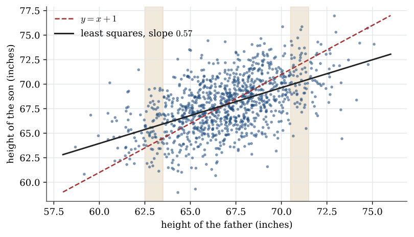
Picture the heights of about a thousand fathers and their adult sons, with the fathers averaging 67 inches and the sons 68 inches. Since sons are one inch taller on average, it is tempting to predict a son’s height as his father’s plus one inch, the line y=x+1. Look at the fathers near 63 inches: most of their sons lie above that line. Near 71 inches, most lie below it. The line through the middle of each vertical strip has slope less than one. That is the regression effect, and finding that line is the job of least squares.
The effect is not a force pulling families towards the mean. When two variables have the same spread and correlation \rho<1, the best linear prediction of one from the other moves only a fraction \rho of the way. Predicting fathers from sons shows the same regression in reverse.
Least squares
Definition 1 (Least-squares line) For points (x_1,y_1),\ldots,(x_n,y_n) with the x_i not all equal, the least-squares line y=b_0+b_1x minimises
L(b_0,b_1)=\sum_{i=1}^n (y_i-b_0-b_1 x_i)^2.
The minimiser is
b_1=\frac{\sum_{i=1}^n(x_i-\overline x)(y_i-\overline y)}{\sum_{i=1}^n(x_i-\overline x)^2}, \qquad b_0=\overline y-b_1\overline x.
Setting \partial L/\partial b_0=0 and \partial L/\partial b_1=0 gives the two normal equations \sum(y_i-b_0-b_1x_i)=0 and \sum x_i(y_i-b_0-b_1x_i)=0. The first gives b_0=\overline y-b_1\overline x, so the line passes through (\overline x,\overline y). Substituting it into the second gives the formula for b_1. The worked answer to the exercise below fills in the algebra.
Example 1 (Advertising and sales) A company records monthly advertising spending x and sales y, both in units of 10 000 dollars.
| Month | 1 | 2 | 3 | 4 | 5 | 6 | 7 | 8 | 9 | 10 |
|---|---|---|---|---|---|---|---|---|---|---|
| Spending x | 1.2 | 0.8 | 1.0 | 1.3 | 0.7 | 0.8 | 1.0 | 0.6 | 0.9 | 1.1 |
| Sales y | 101 | 92 | 110 | 120 | 90 | 82 | 93 | 75 | 91 | 105 |
Question. Find the least-squares line.
Solution. \overline x=0.94 and \overline y=95.9. The sums are \sum(x_i-\overline x)^2=0.444 and \sum(x_i-\overline x)(y_i-\overline y)=23.34, so b_1=23.34/0.444=52.6 and b_0=95.9-52.6\times0.94=46.5. The fitted line is y=46.5+52.6\,x: each extra 10 000 dollars of advertising goes with about 526 000 dollars of extra sales, in these data. The line fits a scatter of past months. It does not say that spending more would cause more sales.
The line is best only for squared vertical deviations. Minimising absolute deviations gives a different line, less sensitive to outliers. Minimising horizontal deviations, to predict x from y, gives yet another. Squared deviations are used because the minimiser has a closed form, and because, under a normal model, least squares is maximum likelihood. If the line must pass through the origin, y=bx, the same calculation gives b=\sum x_iy_i/\sum x_i^2.
Curved relationships
Not every relationship is a straight line. Two remedies keep the least-squares machinery.
The first fits a polynomial, y=b_0+b_1x+\cdots+b_kx^k. The sum of squares is still quadratic in the coefficients, so setting its k+1 partial derivatives to zero gives k+1 linear equations. The model is still linear in its parameters, even though the curve is not a line.
The second transforms the variables. If theory says y=ae^{bx}, then \log y=\log a+bx is linear in x, and a line is fitted to the points (x_i,\log y_i). The same idea linearises y=ax^b, on the log–log scale, and a logistic curve, on the logit scale. The fitted slope is then a slope on the transformed scale, and so are the errors.
Example 2 (Melanoma and latitude) The melanoma rate per 100 000 white males in nine US locations is
| Latitude | 32.8 | 33.9 | 34.1 | 37.9 | 40.0 | 40.8 | 41.7 | 42.2 | 45.0 |
|---|---|---|---|---|---|---|---|---|---|
| Rate | 9.0 | 5.9 | 6.6 | 5.8 | 5.5 | 3.0 | 3.4 | 3.1 | 3.8 |
Question. Compare a straight line, a quadratic and a line for the log rate.
Solution. The straight line is y=20.6-0.399\,x, but the points bend: the southernmost location is far above it. A quadratic fits the bend, y=66.4-2.81\,x+0.0314\,x^2, at the cost of a coefficient with no simple meaning. The log rate is close to linear, \log y=4.51-0.0761\,x, which says the rate falls by a factor e^{-0.0761}=0.93, about 7%, for each degree further north. A constant percentage change per degree is often the more natural reading for a rate.
The normal linear model
Least squares so far is a fit to numbers. It becomes inference when the numbers are treated as a sample. Regard each y_i as the outcome of a random variable Y_i at a fixed value x_i of the explanatory variable, with mean on a line,
\mathbb{E} Y_i=\beta_0+\beta_1x_i,\qquad i=1,\ldots,n.
The line y=\beta_0+\beta_1x is the regression line. Its coefficients are unknown, so it cannot be drawn. The fitted line y=\widehat\beta_0+\widehat\beta_1x is the estimated regression line, and it is not the same thing. The x_i are lower case because they are treated as known and fixed: when the model is used to predict, x is given and Y is not.
Write S_{xx}=\sum(x_i-\overline x)^2, S_{xY}=\sum(x_i-\overline x)(Y_i-\overline Y) and S_{YY}=\sum(Y_i-\overline Y)^2. The least-squares estimators are
\widehat\beta_1=\frac{S_{xY}}{S_{xx}},\qquad\widehat\beta_0=\overline Y-\widehat\beta_1\overline x.
Proposition 1 (Least-squares estimators are unbiased) If \mathbb{E} Y_i=\beta_0+\beta_1x_i for every i, then \mathbb{E}\widehat\beta_1=\beta_1 and \mathbb{E}\widehat\beta_0=\beta_0. No assumption about the error distribution is needed.
Because \sum(x_i-\overline x)=0, the term in \overline Y drops out of S_{xY}, and
\widehat\beta_1=\frac{\sum_{i=1}^n(x_i-\overline x)Y_i}{S_{xx}}.
So \widehat\beta_1 is a linear combination of the Y_i with fixed weights. Taking expectations, and using \sum(x_i-\overline x)=0 again,
\mathbb{E}\sum(x_i-\overline x)Y_i=\sum(x_i-\overline x)(\beta_0+\beta_1x_i)=\beta_1\sum(x_i-\overline x)x_i=\beta_1S_{xx},
so \mathbb{E}\widehat\beta_1=\beta_1. Then \mathbb{E}\overline Y=\beta_0+\beta_1\overline x, and \mathbb{E}\widehat\beta_0=\beta_0+\beta_1\overline x-\beta_1\overline x=\beta_0.
For anything beyond unbiasedness, the errors need a distribution.
Definition 2 (Simple linear regression) The simple linear regression model says
Y_i=\beta_0+\beta_1 x_i+\varepsilon_i, \qquad \varepsilon_i\ \text{independent}\ \operatorname{N}(0,\sigma^2),
with the x_i treated as fixed and not all equal. Equivalently, the Y_i are independent and Y_i\sim\operatorname{N}(\beta_0+\beta_1 x_i,\sigma^2).
The model has three parameters, \beta_0, \beta_1 and \sigma^2. Its likelihood is
L(\beta_0,\beta_1,\sigma^2)=(2\pi\sigma^2)^{-n/2}\exp\Bigl\{-\frac1{2\sigma^2}\sum_{i=1}^n(y_i-\beta_0-\beta_1x_i)^2\Bigr\}.
For any fixed \sigma^2 this is largest when the sum of squares is smallest, so the maximum likelihood estimators of \beta_0 and \beta_1 are the least-squares estimators. The same steps as for a normal sample give the maximum likelihood estimator of the variance, \frac1n\sum(Y_i-\widehat\beta_0-\widehat\beta_1x_i)^2.
Theorem 1 (Sampling distribution of the regression estimators) Under simple linear regression,
\widehat\beta_1\sim\operatorname{N}\Bigl(\beta_1,\ \frac{\sigma^2}{S_{xx}}\Bigr), \qquad \widehat\beta_0\sim\operatorname{N}\Bigl(\beta_0,\ \frac{\sigma^2\sum_ix_i^2}{nS_{xx}}\Bigr),
and with S^2=\frac1{n-2}\sum(Y_i-\widehat\beta_0-\widehat\beta_1x_i)^2,
\frac{(n-2)S^2}{\sigma^2}\sim\chi^2_{n-2},
independently of (\widehat\beta_0,\widehat\beta_1). In particular S^2 is unbiased for \sigma^2. Moreover \widehat\beta_1 and \overline Y are independent.
Article: Sampling distribution of the regression estimators →
\widehat\beta_1 is a fixed linear combination of independent normal variables, so it is normal. Its mean is \beta_1, and its variance is
\operatorname{Var}\widehat\beta_1=\frac{\sum(x_i-\overline x)^2\operatorname{Var} Y_i}{S_{xx}^2}=\frac{\sigma^2}{S_{xx}}.
\widehat\beta_1 and \overline Y are jointly normal, both being linear in the Y_i, so they are independent if they are uncorrelated. Their covariance is
\operatorname{Cov}\Bigl(\frac{\sum(x_i-\overline x)Y_i}{S_{xx}},\ \frac{\sum Y_i}{n}\Bigr)=\frac{\sigma^2}{nS_{xx}}\sum_{i=1}^n(x_i-\overline x)=0.
Then \widehat\beta_0=\overline Y-\overline x\widehat\beta_1 is normal with variance \sigma^2/n+\overline x^2\sigma^2/S_{xx}, and since n\overline x^2+S_{xx}=\sum x_i^2, this is \sigma^2\sum x_i^2/(nS_{xx}). The chi-squared statement is the rotation argument of the normal sample theorem again. Rotate the vector of errors so that two coordinates span the directions (1,\ldots,1) and (x_1-\overline x,\ldots,x_n-\overline x). Those two coordinates determine \widehat\beta_0 and \widehat\beta_1; the remaining n-2 are independent standard normals once divided by \sigma, and their sum of squares is the residual sum of squares over \sigma^2. Two degrees of freedom are spent on the two coefficients.
The maximum likelihood variance estimator divides by n, so its expectation is (n-2)\sigma^2/n; dividing by n-2 removes the bias, as dividing by n-1 does for a single sample. Replacing \sigma^2 by S^2 in the two variances gives the estimated variances S_1^2=S^2/S_{xx} for \widehat\beta_1 and S_0^2=S^2\sum x_i^2/(nS_{xx}) for \widehat\beta_0.
Theorem 2 (Slope t pivot) Under simple linear regression,
\frac{\widehat\beta_1-\beta_1}{S_1}=\frac{\widehat\beta_1-\beta_1}{S/\sqrt{S_{xx}}}
has the t_{n-2} distribution.
Divide the numerator by its standard deviation \sigma/\sqrt{S_{xx}} to get a standard normal Z, and the denominator by the same quantity to get \sqrt{V/(n-2)} with V=(n-2)S^2/\sigma^2\sim\chi^2_{n-2}. By the theorem above, Z and V are independent, so the ratio is t_{n-2}. It follows that
\widehat\beta_1\pm t_{n-2;\,1-\alpha/2}\,S_1
is a confidence interval for \beta_1 with confidence 1-\alpha, and that H_0:\beta_1=0 is rejected against \beta_1\neq0 when |\widehat\beta_1/S_1|\ge t_{n-2;1-\alpha/2}. If \beta_1=0, the model is a single normal sample and x explains nothing.
Example 3 (Heart rate and oxygen intake) For one person, heart rate and oxygen intake are measured together 19 times.
| Heart rate | 94 | 96 | 95 | 95 | 94 | 95 | 94 | 104 | 104 | 106 |
|---|---|---|---|---|---|---|---|---|---|---|
| Oxygen | 0.473 | 0.753 | 0.929 | 0.939 | 0.832 | 0.983 | 1.049 | 1.178 | 1.176 | 1.292 |
| Heart rate | 108 | 110 | 113 | 113 | 118 | 115 | 121 | 127 | 131 |
|---|---|---|---|---|---|---|---|---|---|
| Oxygen | 1.403 | 1.499 | 1.529 | 1.599 | 1.749 | 1.746 | 1.897 | 2.040 | 2.231 |
Question. Fit the regression of oxygen intake on heart rate, give a 95% interval for the slope, and test whether the slope is zero.
Solution. Here \overline x=107.0 and S_{xx}=2518. The fitted line is y=-2.804+0.03865\,x. The residual standard deviation is S=0.1205, so S_1=0.1205/\sqrt{2518}=0.00240 and S_0=0.258. With t_{17;0.975}=2.110, the 95% interval for the slope is
0.03865\pm2.110\times0.00240=(0.0336,\ 0.0437).
It excludes zero. Equivalently, t=0.03865/0.00240=16.1, far beyond 2.110, so H_0:\beta_1=0 is rejected. Each extra beat per minute goes with about 0.039 more units of oxygen.
Fitted values, residuals and explained variation
The fitted values are \widehat y_i=\widehat\beta_0+\widehat\beta_1x_i, and the residuals are y_i-\widehat y_i. A residual is an observable stand-in for the unobservable error \varepsilon_i; the distinction is the one in errors and residuals. S is called the residual standard error.
Without the slope, the model is a single normal sample, whose residual variation is S_{YY}=\sum(Y_i-\overline Y)^2. With it, the residual variation is the residual sum of squares. Writing e_i=(y_i-\overline y)-\widehat\beta_1(x_i-\overline x) and expanding,
\sum e_i^2=S_{YY}-2\widehat\beta_1S_{xY}+\widehat\beta_1^2S_{xx}=S_{YY}-\widehat\beta_1^2S_{xx},
because S_{xY}=\widehat\beta_1S_{xx}. So the line accounts for \widehat\beta_1^2S_{xx} of the total.
Definition 3 (Coefficient of determination) The coefficient of determination of a fitted line is
R^2=\frac{\widehat\beta_1^2S_{xx}}{S_{YY}}=\frac{S_{xY}^2}{S_{xx}S_{YY}},
the proportion of the variation of the y_i about their mean that the line accounts for. It lies in [0,1], and it is the square of the sample correlation coefficient of the pairs.
It lies in [0,1] because the residual sum of squares is between 0 and S_{YY}: least squares cannot do worse than the flat line at \overline y, which is the case b_1=0. For the advertising data R^2=0.77, and for the heart-rate data R^2=0.94. A high R^2 does not show that the relationship is linear, or causal; a curved relationship can have a high R^2 for a line, and a plot of the residuals against x is the check.
The mean response and a new response
Linear regression is often used to say something about Y at a new value x, when Y is hard to measure and x is easy.
The mean response at x is \beta_0+\beta_1x, estimated by
\widehat Y=\widehat\beta_0+\widehat\beta_1x=\overline Y+\widehat\beta_1(x-\overline x).
\overline Y and \widehat\beta_1 are independent and normal, so \widehat Y is normal with mean \beta_0+\beta_1x and variance \sigma^2\{1/n+(x-\overline x)^2/S_{xx}\}. Replacing \sigma by S gives a t_{n-2} pivot, and the confidence interval for the mean response is
\widehat Y\pm t_{n-2;\,1-\alpha/2}\,S\sqrt{\frac1n+\frac{(x-\overline x)^2}{S_{xx}}}.
Definition 4 (Prediction interval) For a new response Y\sim\operatorname{N}(\beta_0+\beta_1x,\sigma^2) independent of the sample, the interval
\widehat Y\pm t_{n-2;\,1-\alpha/2}\,S\sqrt{1+\frac1n+\frac{(x-\overline x)^2}{S_{xx}}}
contains Y with probability 1-\alpha.
A new response has two sources of variation. Y itself varies about the line with variance \sigma^2, and the line has to be estimated. Because the new Y is independent of \widehat Y, the variance of Y-\widehat Y is the sum, \sigma^2\{1+1/n+(x-\overline x)^2/S_{xx}\}, which accounts for the extra 1.
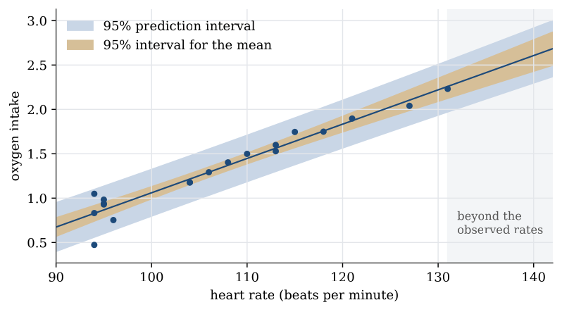
The interval for the mean response shrinks to zero width as n grows. The prediction interval does not: even with the line known exactly, a new Y still has variance \sigma^2. Both widen as x moves away from \overline x, because an error in the slope matters more far from the centre of the data.
For the heart-rate data at x=140 beats per minute, \widehat y=2.607. The 95% interval for the mean oxygen intake is 2.607\pm2.110\times0.0839=(2.43,\ 2.78), and the 95% prediction interval for a single measurement is 2.607\pm2.110\times0.1468=(2.30,\ 2.92). A heart rate of 140 is beyond the largest one observed, 131. Both intervals assume that the line continues to hold out there, which the data cannot check.
A bivariate normal sample
So far the x_i were fixed. If instead the pairs (X_i,Y_i) are a random sample from a two-dimensional distribution, the standard model is the bivariate normal, with means \mu_X,\mu_Y, variances \sigma_X^2,\sigma_Y^2 and correlation \rho. Its density contours are ellipses, the shape of the father–son scatter above.
A bivariate normal pair can be generated from two independent standard normals U and V as
X=\mu_X+\sigma_XU,\qquad Y=\mu_Y+\sigma_Y\bigl(\rho U+\sqrt{1-\rho^2}\,V\bigr).
Substituting U=(X-\mu_X)/\sigma_X shows that, given X=x, Y is normal with mean
\mu_Y+\rho\,\frac{\sigma_Y}{\sigma_X}(x-\mu_X)
and variance \sigma_Y^2(1-\rho^2). The conditional mean is linear in x with slope \rho\sigma_Y/\sigma_X, and the conditional variance does not depend on x. Conditioning on the observed x_i therefore brings this model back to simple linear regression, and the least-squares slope estimates \rho\sigma_Y/\sigma_X. When \sigma_X=\sigma_Y the slope is \rho itself, which is the regression effect in one formula.
The moment estimators of the five parameters are \overline X, \overline Y, S_{XX}/n, S_{YY}/n and the sample correlation R=S_{XY}/\sqrt{S_{XX}S_{YY}}, and these are also the maximum likelihood estimators. Under H_0:\rho=0,
\frac{R\sqrt{n-2}}{\sqrt{1-R^2}}
has the t_{n-2} distribution. It is the slope t statistic of the fixed-x model written in terms of R: since R^2=\widehat\beta_1^2S_{xx}/S_{YY} and (n-2)S^2=S_{YY}(1-R^2), the ratio \widehat\beta_1/S_1 simplifies to exactly this expression.
Example 4 (Testing a correlation) Twenty pairs are generated by computer from a bivariate normal distribution with \mu_X=43, \mu_Y=4, \sigma_X^2=169, \sigma_Y^2=0.25 and \rho=0.4. The estimates from the sample are \widehat\mu_X=43.98, \widehat\mu_Y=3.92, \widehat\sigma_X^2=157.2, \widehat\sigma_Y^2=0.285 and R=0.438.
Question. Test H_0:\rho=0 against \rho\neq0 at level 0.05.
Solution. The statistic is 0.438\sqrt{18}/\sqrt{1-0.438^2}=2.06, against t_{18;0.975}=2.101. It falls just short, with two-sided p-value 0.054, so H_0 is not rejected at the 5% level, although the true correlation is 0.4. Twenty pairs give little power against a moderate correlation. Failing to reject is not evidence that \rho=0.
Least squares chooses the line. The normal model gives the line a sampling distribution, and from that a t interval for the slope, a shorter interval for the mean response, and a longer interval for a new observation.
Further numerical fits, including a regression with two covariates, are in Regression examples.
Questions on this topic
Open a question to attempt it. Its worked answer is folded away at the bottom of the page.
What links here
Pages (7)
- Statistical inference — via Linear regression
- Estimation — via Linear regression
- Analysis of variance — via Linear regression
- Using R — via Linear regression
- Regression examples — via least-squares line, Linear regression, prediction interval, interval for the mean response
- Linear model examples — via Linear regression
- Bayesian linear regression — via Linear regression
Questions and answers (3)
See also
- Articles from this chapter: Least-squares line · Least-squares estimators are unbiased · Simple linear regression · Sampling distribution of the regression estimators · Slope t pivot · Coefficient of determination · Prediction interval
- All statistical inference chapters
- Glossary and index
- Distribution sheet and formula lookup