Probability-integral residuals
Part of Generalised linear models · What links here
Probability-integral residuals
| Part | Generalised linear models |
| Chapter | 6 of 6 in this part |
| Previous | Paired comparisons, and how far a fit is from the data |
| Figures | 1 |
A Pearson plot of a binary or a count fit is striped. The stripes are the values the response is allowed to take, not a missed term. This is the last diagnostic that still belongs with generalised linear models. It replaces that plot with a transform that does not care what the distribution was.
Suppose Y has continuous distribution function F. Then U=F(Y) is uniform on (0,1). The probability of falling below the value you actually observed, scored by the distribution that generated it, is a uniform draw. If F is discrete the same idea uses a generalised inverse, and F(Y) is only approximately uniform. The approximation improves as the fitted distribution spreads over more values. A Bernoulli is the worst case. A Poisson with a large mean is kinder.
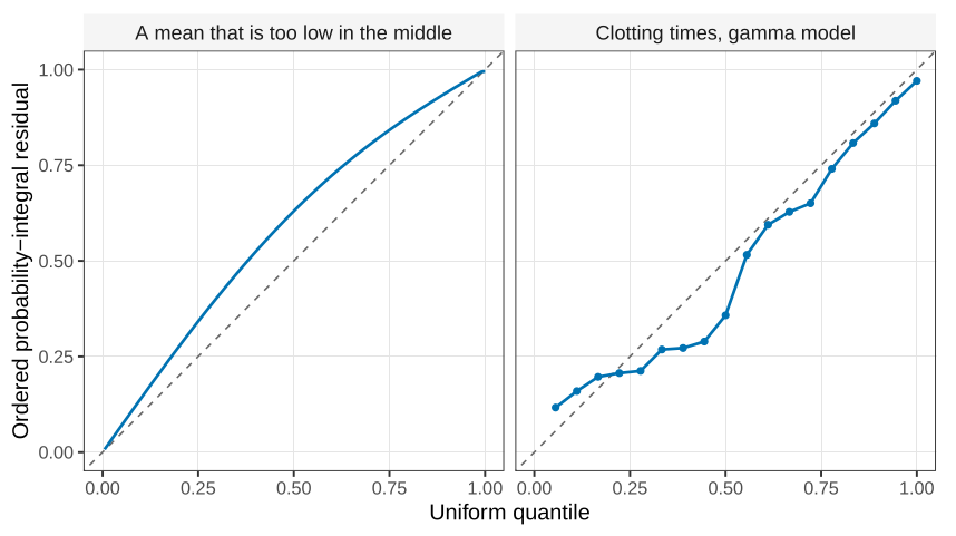
After a model has been fitted, plug in \hat{\boldsymbol{\theta}} and compute F(y_i;\hat{\boldsymbol{\theta}}) for each observation. These are not exactly uniform, for the same reason a residual divided by \hat\sigma is not exactly standard normal: the parameters were estimated. If the model is adequate they should still look like a uniform sample. Order them and plot them against the uniform quantiles 1/n,2/n,\ldots,n/n. Those quantiles are equally spaced, which is the one pleasant feature of the uniform that the normal does not share. A straight line is what you want.
A probability-integral residual asks whether each observation sits where the fitted distribution said it would. The reference distribution is uniform, for a binomial, a Poisson, a gamma, or a normal. You do not first transform the data toward normality.
Bend the line and the fit is wrong in a readable way. If the plotted residuals bow above the diagonal through the middle of the sample, the middle observations are larger than the fitted distribution expected: the mean is too low in the middle of the range. The opposite bow means the fit is too high there. Either shape is a reason to change the mean, not to stare harder at a banded Pearson plot.
The same construction works when the data really are normal. F is then a normal distribution function, and the uniform plot is that normal probability transformed one more time. The classical residual plots remain the right tool when Y is continuous and the variance function is the thing in doubt.
The next question is what to do when no straight line, on any link, is a shape you are willing to write down in advance.
- State what F(Y) is distributed as when F is the true continuous distribution function of Y, and why the plotted reference quantiles for a sample of size n are equally spaced.
What links here
Pages (1)
- Paired comparisons, and how far a fit is from the data — via probability-integral-transform residual