Simulation
Part of Probability · 4 questions on this topic · What links here
Simulation
| Part | Probability |
| Chapter | 3 of 7 in this part |
| Previous | Random variables and distributions |
| Next | Joint distributions |
| Questions | 4 |
| Definitions | Linear congruential generator · Inverse-transform method · Acceptance–rejection method |
| Figures | 2 |
Simulation turns a supply of uniform random numbers into draws from a distribution that has been specified. The two general constructions are the inverse-transform method, which reads the distribution function backwards, and acceptance–rejection, which keeps the draws that land under the target density. Particular families then have shorter algorithms. The families themselves are on the common distributions page, together with the uniform and hypergeometric laws in Random variables and distributions.
Random numbers
Coins, dice and roulette wheels were the first random number generators, and physical devices such as noise diodes and Geiger counters followed. Simulation abandoned them: they are slow, their output cannot be reproduced, and their numbers turn out to be biased and dependent. Almost every generator in use today is a short deterministic recursion whose output passes the statistical tests a truly random sequence would. Such numbers are called pseudorandom.
Definition 1 (Linear congruential generator) A linear congruential generator produces integers by the recursion
X_{i+1}=(aX_i+c)\bmod m,
starting from a seed X_0, with positive integer multiplier a, increment c and modulus m. The pseudorandom numbers are U_i=X_i/m. With c=0 it is a multiplicative congruential generator.
Each X_i lies in \{0,1,\ldots,m-1\}, so the sequence must repeat within m steps: its period is at most m. With a=c=X_0=3 and m=5, the recursion gives 3,2,4,0,3,\ldots, with period 4. Only carefully chosen constants give long periods and good statistical behaviour; a classic choice for 32-bit arithmetic is the multiplicative generator with m=2^{31}-1, a prime, and a=7^5=16807. Modern libraries use longer recursions with periods far beyond any simulation’s needs.
A uniform generator, then, returns numbers that behave as independent draws from \operatorname{U}[0,1]. Setting a seed makes the sequence repeatable: the same seed produces the same stream, which is what lets a simulation be checked and its bugs reproduced. In Python, np.random.seed(1234) followed by np.random.rand(5) returns the same five numbers every time. Every method below assumes such a stream and nothing else.
Inverse transform
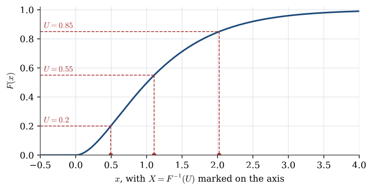
Definition 2 (Inverse-transform method) Let F be a distribution function and define F^{-1}(u)=\inf\{x:F(x)\ge u\} for u\in(0,1). If U\sim\operatorname{U}[0,1], then X=F^{-1}(U) has distribution function F.
The proof is one line when F is continuous and strictly increasing: \mathbb{P}(F^{-1}(U)\le x)=\mathbb{P}(U\le F(x))=F(x).
The general definition, with the infimum, covers flat stretches and jumps. Operationally the algorithm is: draw U from \operatorname{U}[0,1], and return F^{-1}(U).
A density f(x)=2x on [0,1] has distribution function F(x)=x^2 there, so the inverse transform returns \sqrt{U}.
For a discrete variable on points x_1<x_2<\cdots with masses p_i, the distribution function is a step function. Draw U and return the first x_k whose step has reached U, that is the smallest k with U\le F(x_k). If the masses are stored in a vector p, one draw is the first index at which the cumulative sum exceeds U.
The method needs a usable inverse. The exponential, uniform, Weibull, logistic and Cauchy distribution functions invert in closed form. Many others do not, and even a closed inverse can be a poor algorithm if it is expensive to evaluate.
Acceptance and rejection
Definition 3 (Acceptance–rejection method) Suppose the target density f is zero outside a finite interval [a,b] and bounded by c=\max f. Draw X uniformly from [a,b] and, independently, Y uniformly from [0,c]. If Y\le f(X), return X. Otherwise repeat.
The pair (X,Y) is uniform on the rectangle [a,b]\times[0,c]. Keeping the pairs that fall under the graph of f makes the retained X have density proportional to that graph, which is f itself because f integrates to one.
The same idea works with a proposal density g that is easy to sample, provided a constant C\ge 1 majorises the target: f(x)\le C\,g(x) for every x. Draw X from g and, independently, Y uniformly from [0, C g(X)]. Accept X when Y\le f(X). The probability of acceptance is 1/C, the ratio of the area under f to the area under C g. A useful proposal is easy to sample and has C close to 1.
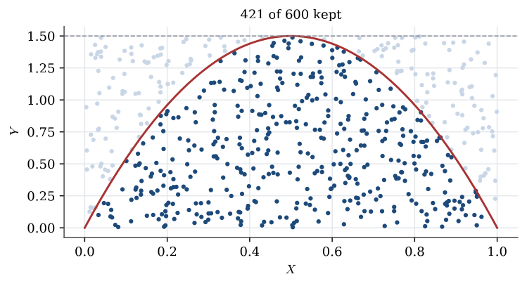
The number of trials until the first acceptance is geometric, starting at 1, with success probability 1/C. For the triangular density f(x)=2x on [0,1], the proposal g=1 on [0,1] needs C=2. Half of the proposals are rejected. The inverse-transform method is the better algorithm for that particular density; rejection is the method that remains when the inverse is unavailable.
Example 1 (Rejection for a beta density) The density f(x)=6x(1-x) on [0,1] is the \operatorname{Beta}(2,2) law.
Question. Describe a rejection sampler with uniform proposals, find its efficiency, and find the expected number of uniform random numbers it uses per accepted draw.
Solution. The density is largest at x=1/2, where f=1.5, so take c=1.5. Draw X\sim\operatorname{U}[0,1] and Y\sim\operatorname{U}[0,1.5], and accept X if Y\le6X(1-X). The acceptance probability is the area under f, which is 1, over the area of the box, 1.5, so the efficiency is 2/3. The number of proposals until acceptance is geometric with mean 1.5, and each proposal uses two uniforms, so on average 3 uniforms are spent per accepted draw.
Draws from the usual families
Exponential. If X\sim\operatorname{Exp}(\lambda), then F(x)=1-e^{-\lambda x} for x>0, so F^{-1}(u)=-\lambda^{-1}\log(1-u). Because 1-U is again uniform on [0,1], the draw X=-\lambda^{-1}\log U has the same distribution. In Python, with numpy imported as np,
u = np.random.rand()
x = -np.log(u) / lam
Uniform on an interval. If U\sim\operatorname{U}[0,1], then a+(b-a)U is uniform on [a,b]. This is the inverse transform of the linear distribution function, and it is also an affine image of a uniform variable.
Normal. There is no elementary inverse of \Phi. If a standard normal draw Z is already available, then \mu+\sigma Z is \operatorname{N}(\mu,\sigma^2). Two independent standard normals can be made from two independent uniforms (U,V) by the Box–Muller map
Z_1=\sqrt{-2\log U}\,\cos(2\pi V), \qquad Z_2=\sqrt{-2\log U}\,\sin(2\pi V).
The Jacobian of that transformation is checked in Functions of random variables and limit theorems. The two coordinates come out independent and standard normal.
Bernoulli and binomial. A Bernoulli trial with success probability p is the indicator \mathbf{1}\{U\le p\}. A binomial count is the sum of n independent copies. That uses the representation of the binomial distribution as a sum of Bernoulli trials, rather than an inverse of its distribution function.
Geometric and Poisson. A geometric count starting at 1, with success probability p, is the number of Bernoulli trials until the first success, which is \lfloor \log U/\log(1-p)\rfloor+1. A Poisson count can be built from exponential spacings: if E_i are independent exponential variables with rate 1, the largest n with E_1+\cdots+E_n\le\lambda is Poisson with mean \lambda. Both constructions are consequences of the memoryless property and of the gamma–Poisson relationship, not new definitions of the laws.
Discrete distributions in general. Stack the masses into a cumulative sum and apply the discrete inverse transform. That one algorithm covers every finite support, including an empirical distribution read off a table.
One uniform draw, passed through F^{-1}, has distribution function F. When the inverse is awkward, propose from a density that sits above f and keep the proposals that fall underneath it. The chance of keeping a proposal is 1/C.
Questions on this topic
Open a question to attempt it. Its worked answer is folded away at the bottom of the page.
What links here
Pages (4)
- Random variables and distributions — via simulation
- Functions of random variables and limit theorems — via inverse-transform method, Box–Muller, Simulation
- Markov chains — via inverse-transform method
- Studies, data, and evidence — via Simulation
Questions and answers (1)
- Draws from an exponential law (answer)
See also
- Articles from this chapter: Linear congruential generator · Inverse-transform method · Acceptance–rejection method
- All probability chapters
- Glossary and index
- Distribution sheet and formula lookup