Joint distributions
Part of Probability · 8 questions on this topic · What links here
Joint distributions
| Part | Probability |
| Chapter | 4 of 7 in this part |
| Previous | Simulation |
| Next | Functions of random variables and limit theorems |
| Questions | 8 |
| Definitions | Joint probability mass function · Independent random variables · Joint probability density · Covariance · Expectation vector and covariance matrix · Conditional distribution |
| Results | Tower property |
| Figures | 2 |
Two or more random variables on the same experiment have a joint distribution. The joint distribution determines the individual distributions, the probability of any region in the plane or in a higher dimension, and the conditional distribution of one variable given the others. Independence is the special case in which the joint distribution is the product of the marginals.
Conditional probability for events is in Random experiments and probability. The density form used to update a prior is Bayes’ rule. The named one-dimensional families are on the common distributions page.
Joint distributions and independence
Definition 1 (Joint probability mass function) Discrete random variables X and Y have joint probability mass function f_{X,Y}(x,y)=\mathbb{P}(X=x,Y=y). The marginal mass functions are the row and column sums,
f_X(x)=\sum_y f_{X,Y}(x,y), \qquad f_Y(y)=\sum_x f_{X,Y}(x,y).
For any set B of pairs, \mathbb{P}((X,Y)\in B)=\sum_{(x,y)\in B}f_{X,Y}(x,y). The definition extends to any finite collection by using the probability of the whole tuple.
Definition 2 (Independent random variables) Discrete random variables X_1,\ldots,X_n are independent when the joint mass function factors for every point:
\mathbb{P}(X_1=x_1,\ldots,X_n=x_n)=\prod_{k=1}^n \mathbb{P}(X_k=x_k).
Continuous random variables with joint density f are independent when f(x_1,\ldots,x_n)=\prod_{k=1}^n f_{X_k}(x_k). An infinite sequence is independent when every finite subcollection is.
Independence of the random variables is independence of the events \{X_i\in A_i\} for every choice of measurable sets A_i. It is a property of the joint distribution, and it is usually put in as a modelling assumption. A box of dice, one of which is biased, does not give independent rolls if the die is first chosen at random and then rolled twice: the first roll carries information about which die was chosen. Two rolls of a single fair die are independent.
Example 1 (A box of three dice) A box holds three dice. Die 1 is ordinary. Die 2 has no six but two fives. Die 3 has no five but two sixes. A die is chosen at random and thrown. Let X be the number of the die and Y the face shown.
Question. Find the joint mass function and both marginals. Are X and Y independent?
Solution. Each die is chosen with probability 1/3, and each of its six faces then shows with probability 1/6, so each face position has probability 1/18. A value printed on two faces gets 2/18=1/9.
| y=1 | y=2 | y=3 | y=4 | y=5 | y=6 | f_X(x) | |
|---|---|---|---|---|---|---|---|
| x=1 | 1/18 | 1/18 | 1/18 | 1/18 | 1/18 | 1/18 | 1/3 |
| x=2 | 1/18 | 1/18 | 1/18 | 1/18 | 1/9 | 0 | 1/3 |
| x=3 | 1/18 | 1/18 | 1/18 | 1/18 | 0 | 1/9 | 1/3 |
| f_Y(y) | 1/6 | 1/6 | 1/6 | 1/6 | 1/6 | 1/6 | 1 |
The marginals are the row and column sums. Remarkably, Y is uniform on \{1,\ldots,6\}, exactly as for a single fair die. Yet X and Y are not independent: \mathbb{P}(X=2,Y=6)=0, while f_X(2)f_Y(6)=1/18. Seeing a six rules out die 2. The marginals alone cannot reveal the dependence; only the joint table can.
The multinomial distribution is the joint law of independent trials with several outcomes. In n independent trials, each falling in category k with probability p_k, the vector of counts is multinomial. Its mass function, mean and coordinate-wise variance are on the distribution sheet. One coordinate of a multinomial vector is binomial, because collapsing every other category leaves a single success probability.
Definition 3 (Joint probability density) Continuous random variables X and Y have joint density f when, for every reasonable region B,
\mathbb{P}((X,Y)\in B)=\iint_B f(x,y)\,\,\mathrm{d} x\,\,\mathrm{d} y.
The marginal density of X is f_X(x)=\int f(x,y)\,\,\mathrm{d} y.
Probability is volume under the surface f. A point drawn uniformly from a region of area a has joint density 1/a on that region. Two independent uniform draws on [0,1] have joint density 1 on the unit square, which is the product of the marginal densities.
A random sample of size n from a density f is exactly this product situation: X_1,\ldots,X_n independent, each with density f, so the joint density is \prod_{i=1}^n f(x_i).
Expectation, covariance and matrices
For a function g of a discrete pair, \mathbb{E} g(X,Y)=\sum_{x,y} g(x,y)\,f_{X,Y}(x,y). For a continuous pair the sum is an integral against the joint density. In particular, expectation is still linear without any independence assumption:
\mathbb{E}(aX+bY)=a\,\mathbb{E} X+b\,\mathbb{E} Y.
The product factors only under independence: if X and Y are independent and the expectations exist, then \mathbb{E}(XY)=(\mathbb{E} X)(\mathbb{E} Y).
This is why a binomial expectation is np. Write the count as a sum of n independent Bernoulli indicators. Each has expectation p, and linearity gives np. The same argument gives the hypergeometric mean np, with p=r/N, even though those indicators are dependent: linearity does not ask them to be independent. The variance does feel the dependence, which is why the hypergeometric variance carries the factor (N-n)/(N-1).
Sums stay inside several families, and the moment generating function is the clean way to see it. If X\sim\operatorname{Poisson}(\lambda) and Y\sim\operatorname{Poisson}(\mu) are independent, then M_X(s)=\exp(\lambda(e^s-1)) and M_{X+Y}(s)=\exp((\lambda+\mu)(e^s-1)), which is the transform of \operatorname{Poisson}(\lambda+\mu). Independent gamma variables with a common rate \lambda and shapes \alpha and \beta add to a gamma variable with shape \alpha+\beta and the same rate, because the transforms (\lambda/(\lambda-s))^{\alpha} multiply.
Definition 4 (Covariance) The covariance of X and Y is \operatorname{Cov}(X,Y)=\mathbb{E}\bigl((X-\mathbb{E} X)(Y-\mathbb{E} Y)\bigr), when the expectation exists. Equivalently, \operatorname{Cov}(X,Y)=\mathbb{E}(XY)-(\mathbb{E} X)(\mathbb{E} Y).
Covariance is bilinear and symmetric, and \operatorname{Cov}(X,X)=\operatorname{Var}(X). The variance of a sum expands as
\operatorname{Var}(X+Y)=\operatorname{Var}(X)+\operatorname{Var}(Y)+2\operatorname{Cov}(X,Y).
Independent variables with finite variances are uncorrelated: their covariance is zero. The converse is false. Uncorrelated variables can be dependent. For jointly normal variables the converse does hold, which is proved with the transformation rule in the next chapter.
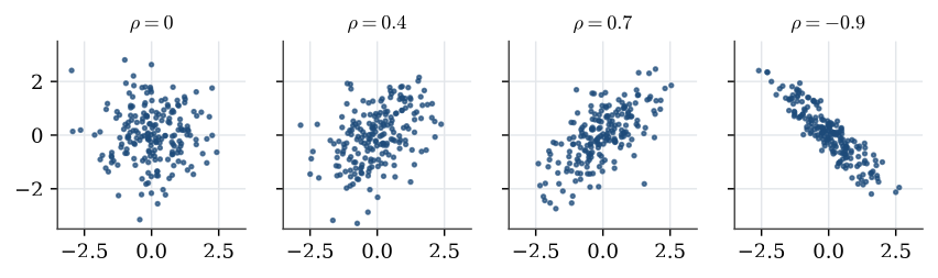
The correlation \rho(X,Y)=\operatorname{Cov}(X,Y)/\sqrt{\operatorname{Var}(X)\operatorname{Var}(Y)} lies in [-1,1] whenever the variances are positive and finite. Equality to \pm 1 means that one variable is an affine function of the other. The bound is the Cauchy–Schwarz inequality applied to the centred variables, or equivalently the fact that \operatorname{Var}(X+tY)\ge 0 for every real t.
A binomial variance is np(1-p) because the Bernoulli indicators are independent, so the covariances vanish and the variances p(1-p) add. A hypergeometric variance keeps the non-zero covariances of the without-replacement indicators, and they produce the finite-population correction.
Definition 5 (Expectation vector and covariance matrix) For a random column vector \mathbf{X}=(X_1,\ldots,X_n)^\top the expectation vector is \boldsymbol\mu=\mathbb{E}\mathbf{X}, taken coordinate-wise, and the covariance matrix \Sigma has entries \Sigma_{ij}=\operatorname{Cov}(X_i,X_j).
The matrix \Sigma is symmetric. It is positive semidefinite: for every constant vector \mathbf{u},
\mathbf{u}^\top\Sigma\mathbf{u}=\operatorname{Var}(\mathbf{u}^\top\mathbf{X})\ge 0.
In matrix form, \Sigma=\mathbb{E}\bigl((\mathbf{X}-\boldsymbol\mu)(\mathbf{X}-\boldsymbol\mu)^\top\bigr).
Conditional distributions
Definition 6 (Conditional distribution) If X and Y are both discrete or both continuous, and f_X(x)>0, the conditional mass function or density of Y given X=x is
f_{Y\mid X}(y\mid x)=\frac{f_{X,Y}(x,y)}{f_X(x)}.
In the discrete case this is ordinary conditional probability: \mathbb{P}(Y=y\mid X=x)=\mathbb{P}(X=x,Y=y)/\mathbb{P}(X=x). In the continuous case the same ratio is the density of the conditional distribution function \mathbb{P}(Y\le y\mid x<X\le x+h) as h\downarrow 0.
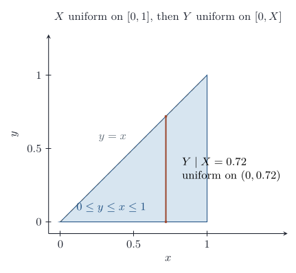
Rearrangement is the product rule for densities, f_{X,Y}(x,y)=f_X(x)\,f_{Y\mid X}(y\mid x). Integrating out x is the law of total probability for densities,
f_Y(y)=\int f_{Y\mid X}(y\mid x)\,f_X(x)\,\,\mathrm{d} x.
The conditional expectation \mathbb{E}(Y\mid X=x) is the expectation of Y under that conditional distribution. As a function of the random point X it is a random variable, written \mathbb{E}(Y\mid X).
Example 3 (A uniform point on a triangle) A point (X,Y) is drawn uniformly from the 10 lattice points with 1\le x\le y\le4, so each has probability 1/10.
Question. Find the marginals, the conditional distribution of Y given X=x, and \mathbb{E}(Y\mid X). Check the tower property, and find the correlation.
Solution. For a given x there are 5-x admissible values of y, and for a given y there are y values of x, so
f_X(x)=\frac{5-x}{10},\qquad f_Y(y)=\frac{y}{10},\qquad x,y\in\{1,2,3,4\}.
X and Y are dependent: given X=2, Y can only be 2, 3 or 4. The conditional mass function is
f_{Y\mid X}(y\mid x)=\frac{1/10}{(5-x)/10}=\frac1{5-x},\qquad y=x,\ldots,4,
uniform on the admissible values. So \mathbb{E}(Y\mid X=x)=(x+4)/2. Averaging over X,
\mathbb{E}\bigl(\mathbb{E}(Y\mid X)\bigr)=\tfrac52\cdot\tfrac4{10}+3\cdot\tfrac3{10}+\tfrac72\cdot\tfrac2{10}+4\cdot\tfrac1{10}=3,
which agrees with \mathbb{E} Y=(1+4+9+16)/10=3. For the correlation, \mathbb{E} X=2, \mathbb{E}(XY)=13/2 and both variances are 1, so \operatorname{Cov}(X,Y)=13/2-6=1/2 and \rho(X,Y)=1/2. A larger X forces a larger Y.
Theorem 1 (Tower property) If the expectations exist, then \mathbb{E}\bigl(\mathbb{E}(Y\mid X)\bigr)=\mathbb{E} Y. More generally, \mathbb{E}\bigl(\mathbb{E}(Y\mid X,Z)\mid X\bigr)=\mathbb{E}(Y\mid X).
The tower property is the calculation that justifies “first condition, then average”. A random sum is the standard example. Let N be a count with a finite mean, and given N=n let Y=X_1+\cdots+X_n with the X_i independent of N and of each other, each with mean \mu. Then \mathbb{E}(Y\mid N)=N\mu, so \mathbb{E} Y=\mu\,\mathbb{E} N. The same conditioning gives \operatorname{Var}(Y)=\mathbb{E}(N)\operatorname{Var}(X_1)+\operatorname{Var}(N)(\mathbb{E} X_1)^2 when the variances exist.
Example 4 (A day of takings) A shop has N\sim\operatorname{Poisson}(20) customers a day. Customers spend independently of one another and of N, each with mean 30 dollars and standard deviation 10 dollars.
Question. Find the mean and standard deviation of the day’s takings.
Solution. The takings are a random sum Y=X_1+\cdots+X_N. By the tower property, \mathbb{E} Y=\mu\,\mathbb{E} N=30\times20=600 dollars. For the variance, \operatorname{Var}(N)=20 for a Poisson count, so
\operatorname{Var}(Y)=\mathbb{E}(N)\operatorname{Var}(X_1)+\operatorname{Var}(N)(\mathbb{E} X_1)^2=20\times100+20\times900=20000,
and the standard deviation is 141 dollars. Most of the variability comes from the number of customers, not from what each one spends: if N were fixed at 20, the standard deviation would be only \sqrt{2000}=45 dollars.
The joint distribution is the whole model. Marginals are sums or integrals of it. Independence is factorisation. Covariance is the numerical trace of dependence that variance of a sum can see, and conditional distributions are the joint divided by the marginal.
Questions on this topic
Open a question to attempt it. Its worked answer is folded away at the bottom of the page.
What links here
Pages (11)
- Functions of random variables and limit theorems — via Joint distributions, joint density, covariance
- Statistical inference — via Joint distributions, joint density
- Estimation — via joint density
- Hypothesis tests — via covariance
- Chi-squared tests — via Joint distributions
- Bayesian foundations — via joint density
- Conjugate analysis for normal models — via joint density
- Markov chains, Gibbs sampling, and Metropolis–Hastings — via joint density
- Bayesian hypotheses and model comparison — via joint density
- Exponential families and conjugacy — via joint density
- Hierarchical Bayes — via joint density
Questions and answers (19)
- A joint table · A probability as an integral · A product density · A point in a triangle · Signs and their sum · Sum and proportion of two exponentials · A bivariate-normal Gibbs sampler (answer) · A normal statistic · Q4 · Q9 (answer) · Q18 (answer) · Q23 (answer) · Q25 · Q26 · Q58 (answer) · Question 6 · Question 9 · Question 16 (answer) · Question 17
See also
- Articles from this chapter: Joint probability mass function · Independent random variables · Joint probability density · Covariance · Expectation vector and covariance matrix · Conditional distribution · Tower property
- All probability chapters
- Glossary and index
- Distribution sheet and formula lookup