Chi-squared tests
Part of Statistical inference · 4 questions on this topic · What links here
Chi-squared tests
| Part | Statistical inference |
| Chapter | 5 of 7 in this part |
| Previous | Hypothesis tests |
| Next | Linear regression |
| Questions | 4 |
| Definitions | Pearson statistic · Chi-squared test of independence |
| Results | Pearson chi-squared approximation · Pearson test with estimated parameters |
| Figures | 1 |
A chi-squared statistic compares observed counts with the counts a model expected. It is the large-sample test for a fully specified discrete distribution, for a discrete distribution with a few unknown parameters, and for independence in a contingency table. The likelihood-ratio version of a comparison between nested models is the deviance, developed with paired comparisons and deviance. A contingency table is also the data layout of a categorical response.
The counts themselves are multinomial. That joint distribution is on the common distributions page, and the underlying independence of trials is in Joint distributions. The chi-squared law is defined in Statistical inference.
Counts in categories
Throw n balls independently into k urns, each ball landing in urn i with probability p_i. The numbers (X_1,\ldots,X_k) in the urns are multinomial:
\mathbb{P}(X_1=x_1,\ldots,X_k=x_k)=\frac{n!}{x_1!\cdots x_k!}\,p_1^{x_1}\cdots p_k^{x_k},\qquad x_1+\cdots+x_k=n.
Each X_i is \operatorname{Bin}(n,p_i) on its own, so \mathbb{E} X_i=np_i. The counts are not independent, because they must add to n. Data become multinomial whenever individuals are sorted into classes.
Example 1 (Army recruits by IQ class) Suppose recruits’ IQ scores are \operatorname{N}(100,16^2), and recruits are classed as 1 (IQ at most 90), 2 (between 90 and 110) or 3 (above 110).
Question. Of 7 new recruits, what is the probability that 2 are in class 1, 4 in class 2 and 1 in class 3?
Solution. The class probabilities are p_1=\Phi\{(90-100)/16\}=\Phi(-0.625)=0.266, p_3=0.266 by symmetry, and p_2=0.468. The class counts are \operatorname{Multinomial}(7;\,0.266,0.468,0.266), so
\mathbb{P}(X_1=2,X_2=4,X_3=1)=\frac{7!}{2!\,4!\,1!}\,0.266^2\times0.468^4\times0.266=0.095.
Known cell probabilities
Definition 1 (Pearson statistic) Let (X_1,\ldots,X_k) be multinomial with n trials and cell probabilities p_1,\ldots,p_k. For reference probabilities \pi_1,\ldots,\pi_k the Pearson statistic is
T=\sum_{i=1}^k\frac{(X_i-n\pi_i)^2}{n\pi_i}=\sum_{i=1}^k\frac{(O_i-E_i)^2}{E_i},
where O_i is the observed count and E_i=n\pi_i is the expected count.
Theorem 1 (Pearson chi-squared approximation) If p_i=\pi_i for every i, the Pearson statistic T has approximately the \chi^2_{k-1} distribution for large n.
The case k=2 shows where the k-1 comes from. With two cells, X_2=n-X_1 and \pi_2=1-\pi_1, so X_2-n\pi_2=-(X_1-n\pi_1), and
T=(X_1-n\pi_1)^2\Bigl(\frac1{n\pi_1}+\frac1{n(1-\pi_1)}\Bigr)=\frac{(X_1-n\pi_1)^2}{n\pi_1(1-\pi_1)}=Z^2,
where Z is the standardised binomial count. By the central limit theorem Z is approximately standard normal, so T is approximately \chi^2_1. Two cells give one free squared normal, because the constraint X_1+X_2=n ties the second cell to the first. For general k, the vector of standardised counts is approximately normal by the multivariate central limit theorem, and the constraint \sum X_i=n confines it to a (k-1)-dimensional subspace; the sum of squares there is \chi^2_{k-1}.
The approximation needs every expected count to be large. A usual rule of thumb asks for E_i\ge5 in every cell. Classes with small expected counts are merged before the test is done. The test rejects for large T: at level \alpha, when T\ge\chi^2_{k-1;1-\alpha}. The alternative is simply that the reference probabilities are wrong, in any way at all.
Example 2 (Frizzled chickens) Genetic theory predicts that chickens of types FF, Ff and ff, which are extremely frizzled, slightly frizzled and normal, occur in proportions 1:2:1. Of 93 chickens, 23, 50 and 20 are of the three types.
Question. Are the counts consistent with the theory, at level 0.05?
Solution. The counts are \operatorname{Multinomial}(93;\,p_1,p_2,p_3). Test H_0:(p_1,p_2,p_3)=(1/4,1/2,1/4). The expected counts are 23.25, 46.5 and 23.25, and
T=\frac{(23-23.25)^2}{23.25}+\frac{(50-46.5)^2}{46.5}+\frac{(20-23.25)^2}{23.25}=0.003+0.263+0.454=0.72,
on 3-1=2 degrees of freedom. The critical value is \chi^2_{2;0.95}=5.991, and the p-value is 0.70. The counts are consistent with the 1:2:1 theory.
Estimated parameters
Often the model fixes the form of the cell probabilities but not their values. A count of houses per plot might be Poisson with unknown mean. Then p_i=p_i(\theta) for an unknown r-dimensional parameter \theta, and the expected counts must themselves be estimated.
Theorem 2 (Pearson test with estimated parameters) Let (X_1,\ldots,X_k) be multinomial with cell probabilities p_i(\theta), where \theta has r free coordinates. If \widehat\theta is the maximum likelihood estimator of \theta from the counts and \widehat p_i=p_i(\widehat\theta), then
\sum_{i=1}^k\frac{(X_i-n\widehat p_i)^2}{n\widehat p_i}
is approximately \chi^2_{k-1-r} for large n.
Each freely estimated parameter spends a degree of freedom. The fitted expectations are pulled towards the observed counts by the estimation, so the statistic is smaller than it would be with the true \theta. Using k-1 degrees of freedom anyway, as though \theta were known, makes the test too reluctant to reject.
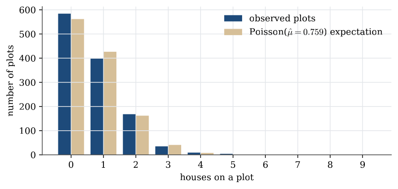
Example 3 (Houses on a village grid) A village of 12 square kilometres is divided into 1200 plots, and the 911 houses are counted plot by plot. If houses are placed at random, the count on a plot should be Poisson.
| Houses on a plot | 0 | 1 | 2 | 3 | 4 | 5 | 6 | 7 | 8 | 9 |
|---|---|---|---|---|---|---|---|---|---|---|
| Plots | 584 | 398 | 168 | 35 | 9 | 4 | 0 | 1 | 0 | 1 |
Question. Test whether the counts per plot are Poisson.
Solution. The maximum likelihood estimate of the Poisson mean is the average count, \widehat\mu=911/1200=0.7592. The fitted expected number of plots with i houses is 1200\,e^{-\widehat\mu}\widehat\mu^{\,i}/i!: 561.67, 426.40, 161.85 and 40.96 for 0 to 3 houses, then 7.77, 1.18 and less than 0.2 after that. To keep every expectation at least 5, merge 4 or more houses into one class, with observed count 15 and expected count 9.12. With k=5 classes and r=1 estimated parameter,
T=\frac{(584-561.67)^2}{561.67}+\frac{(398-426.40)^2}{426.40}+\frac{(168-161.85)^2}{161.85}+\frac{(35-40.96)^2}{40.96}+\frac{(15-9.12)^2}{9.12}=7.67
on 5-1-1=3 degrees of freedom. Since \chi^2_{3;0.95}=7.815, the test just fails to reject at the 5% level; the p-value is 0.053. Most of the statistic comes from the merged tail class: there are more crowded plots, and fewer plots with a single house, than a Poisson law allows. The evidence that houses are not placed at random is suggestive, not conclusive.
Contingency tables
A contingency table classifies n individuals by two factors, with r rows and c columns. Write O_{ij} for the count in row i and column j, R_i for the row total and C_j for the column total. If the individuals are sampled independently, the rc cell counts are multinomial with cell probabilities p_{ij}.
Independence of the two factors says that each cell probability factors into a row probability times a column probability, H_0:p_{ij}=a_ib_j for all i,j. The maximum likelihood estimates are the row and column proportions, \widehat a_i=R_i/n and \widehat b_j=C_j/n, so the fitted count under independence is
E_{ij}=n\,\widehat a_i\widehat b_j=\frac{R_i\,C_j}{n}.
Definition 2 (Chi-squared test of independence) For an r\times c contingency table with fitted counts E_{ij}=R_iC_j/n, the statistic
T=\sum_{i=1}^r\sum_{j=1}^c\frac{(O_{ij}-E_{ij})^2}{E_{ij}}
is approximately \chi^2_{(r-1)(c-1)} when the row and column factors are independent. Large values are evidence against independence.
The degrees of freedom are counted as before. There are rc cells, so rc-1 to start with. The row probabilities sum to one, so r-1 of them are free, and similarly c-1 column probabilities. That leaves rc-1-(r-1)-(c-1)=(r-1)(c-1).
Example 4 (Belief in ESP) A survey asks 114 artists and 344 non-artists how strongly they believe in extra-sensory perception.
| Strong | Moderate | None | Total | |
|---|---|---|---|---|
| Artists | 67 | 41 | 6 | 114 |
| Non-artists | 129 | 183 | 32 | 344 |
| Total | 196 | 224 | 38 | 458 |
Question. Is belief in ESP independent of being an artist?
Solution. The fitted counts are R_iC_j/458. For artists with strong belief, 114\times196/458=48.79; the six fitted counts are
| Strong | Moderate | None | |
|---|---|---|---|
| Artists | 48.79 | 55.76 | 9.46 |
| Non-artists | 147.21 | 168.24 | 28.54 |
The six contributions (O_{ij}-E_{ij})^2/E_{ij} are 6.80, 3.91, 1.27, 2.25, 1.29 and 0.42, so T=15.94 on (2-1)(3-1)=2 degrees of freedom. The p-value is 0.0003. Independence is firmly rejected. The largest contributions come from artists: more of them hold strong belief, and fewer moderate belief, than independence predicts.
A 2\times2 table is a comparison of two proportions. With rows as groups and columns as success and failure, the Pearson statistic equals the square of the two-proportion z statistic with the pooled standard error, and \chi^2_1 is the law of a squared standard normal. The two tests are the same test, except that the chi-squared version is automatically two-sided.
The same table can be read as a response model, with one factor the response and the other the covariate. The saturated log-linear or multinomial-logit fit, and the likelihood-ratio comparison with the independence model, belong to the categorical and deviance chapters rather than to a second copy of this statistic.
Expected counts come from the hypothesis. The Pearson statistic is the sum of squared differences divided by those expectations. The degrees of freedom are the number of free cells left after every estimated parameter has been counted.
Numerical examples are in Chi-squared examples.
Questions on this topic
Open a question to attempt it. Its worked answer is folded away at the bottom of the page.
What links here
Pages (4)
- Random variables and distributions — via Chi-squared tests
- Statistical inference — via Chi-squared tests
- Descriptive statistics — via chi-squared test of independence
- Chi-squared examples — via test of independence, Chi-squared tests
Questions and answers (1)