Descriptive statistics
Part of Data analysis · 2 questions on this topic · What links here
Descriptive statistics
| Part | Data analysis |
| Chapter | 2 of 9 in this part |
| Previous | Studies, data, and evidence |
| Next | Using R |
| Questions | 2 |
| Definitions | Sample quantile · Interquartile range · Sample variance and standard deviation · Five-number summary and boxplot · Normal quantile plot |
| Figures | 5 |
Descriptive statistics summarise a sample before a model is fitted. They show the range, the shape, the odd points, and which variables move together. They do not by themselves test a hypothesis or produce a confidence interval. Those steps are in Statistical inference. The shapes being summarised are the laws on the common distributions page. How the sample was obtained, and whether a pattern can be read causally, is in Studies, data, and evidence.
The running example is a study of 299 patients after heart failure, all with severe weakness of the left ventricle, admitted to one hospital and followed for up to a year. For each patient there are 13 measurements, and the questions are which of them go with death during follow-up, and which go with the ejection fraction, the fraction of the blood in the left ventricle pumped out at each beat. The R code that produces each summary is shown with it; reading data and drawing plots in R is covered in Using R.
The table
One row is one unit. One column is one variable. An identifier column names the unit. In a designed experiment some columns record the assignment and stay fixed if the measurements are repeated. The remaining columns are what the study measured.
| Variable | Meaning | Type |
|---|---|---|
age |
age in years | quantitative |
anaemia |
low red blood cell count, 1 = yes | categorical |
cp |
creatine phosphokinase in the blood, mcg/L | quantitative |
diabetes |
diabetes, 1 = yes | categorical |
ejection_fraction |
percentage of blood leaving the heart at each beat | quantitative |
hbp |
high blood pressure, 1 = yes | categorical |
platelets |
platelets in the blood, kiloplatelets/mL | quantitative |
serum_creatinine |
creatinine in the blood, mg/dL | quantitative |
serum_sodium |
sodium in the blood, mEq/L | quantitative |
sex |
1 = male, 0 = female | categorical |
smoking |
smoker, 1 = yes | categorical |
time |
follow-up period, days | quantitative |
death |
died during follow-up, 1 = yes | categorical |
The follow-up time is not a variable to explain death with. A patient who died was recorded at the time of death, so time is partly determined by the outcome itself; using it to predict death would be circular. It is left out of the analysis.
Variables come in two broad types. Quantitative variables are numbers on a scale where arithmetic makes sense: they are discrete when they count something and continuous when they measure. Categorical variables, called factors in R, put each unit in one of a fixed set of classes; they are ordinal when the classes have a natural order, such as “mild, moderate, severe”, and nominal otherwise. A categorical variable coded as 0 and 1 is still categorical, and R must be told so, or it will happily compute the mean of sex:
heart <- read.csv("heart.csv")
heart$anaemia <- factor(heart$anaemia)   # and likewise for the other 0/1 columns
str(heart)                               # 299 obs. of 13 variables
Summary statistics
For data x_1,\ldots,x_n, the sample mean \overline x=\frac1n\sum x_i is the average and the sample median is the middle value of the sorted data, or the average of the two middle values when n is even. The median is robust: a single wild value can move the mean anywhere but barely moves the median.
Definition 1 (Sample quantile) A sample p-quantile, for 0<p<1, is a value q_p such that a fraction p of the data is at most q_p. The 0.25, 0.5 and 0.75 quantiles are the first quartile, the median and the third quartile; the p-quantile is also the 100pth percentile.
When no data value sits exactly at the fraction p, software interpolates between neighbours. R’s default, used throughout, puts q_p at position 1+(n-1)p of the sorted data, interpolating linearly.
Definition 2 (Interquartile range) The interquartile range is the difference between the third and first quartiles. It is the width of the central half of the sample.
Definition 3 (Sample variance and standard deviation) The sample variance is s^2=\frac1{n-1}\sum_{i=1}^n(x_i-\overline x)^2, and the sample standard deviation is s=\sqrt{s^2}, in the units of the data.
The divisor n-1 makes s^2 an unbiased estimator of the population variance; the reason is in Statistical inference. The range, largest minus smallest, is the crudest measure of spread, and it can only grow as more data arrive.
Example 1 (The ages of 299 patients) Question. Summarise the patients’ ages.
Solution.
mean(heart$age); median(heart$age)     # 60.83  60
quantile(heart$age, c(0.25, 0.75))     # 51  70
IQR(heart$age)                          # 19
sd(heart$age)                           # 11.89
range(heart$age)                        # 40  95
The patients are aged 40 to 95. The mean and median are close, 60.8 and 60, so the ages are roughly symmetric. The middle half lies between 51 and 70, an interquartile range of 19 years, and the standard deviation is 11.9 years. For a roughly normal sample the interquartile range is about 1.35 standard deviations; here 19/11.9=1.6, so the ages are a little flatter than normal.
One categorical variable, and two
A categorical variable is summarised by counts, or by proportions. Of the 299 patients, 96 died during follow-up, a proportion of 0.32.
Two categorical variables are summarised by a contingency table: counts for every combination of categories.
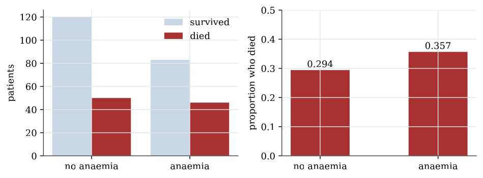
Example 2 (Anaemia and death) Question. Did patients with anaemia die more often?
Solution.
table(heart$anaemia, heart$death, dnn = c("anaemia", "death"))
proportions(table(heart$anaemia, heart$death), margin = 1)| Survived | Died | Proportion died | |
|---|---|---|---|
| No anaemia | 120 | 50 | 0.294 |
| Anaemia | 83 | 46 | 0.357 |
Row proportions, margin = 1, compare the death rate within each anaemia group: 29.4% without anaemia and 35.7% with it. The difference is six percentage points. Whether that is more than chance would produce with groups this size is a chi-squared test of independence, and it is not: the p-value is 0.25. High blood pressure gives 29.4% against 37.1%, with p-value 0.17, while for diabetes, sex and smoking the rates in the two groups differ by less than two percentage points.
A bar plot shows counts or proportions by bars of proportional length. Side-by-side bars of counts mislead when the groups are of different sizes, which is why the proportions within each group are usually the plot to draw. A pie chart shows the same proportions as angles, which the eye compares less accurately than lengths.
One quantitative variable
A quantitative variable is summarised by its shape as well as its centre and spread. The serum creatinine levels, a measure of kidney function, show why.
Definition 4 (Five-number summary and boxplot) The five-number summary of a sample is its minimum, first quartile, median, third quartile and maximum. A boxplot draws the box from the first to the third quartile with a line at the median, and whiskers out to the most extreme data within 1.5 interquartile ranges of the box. Points beyond the whiskers are drawn individually as possible outliers.
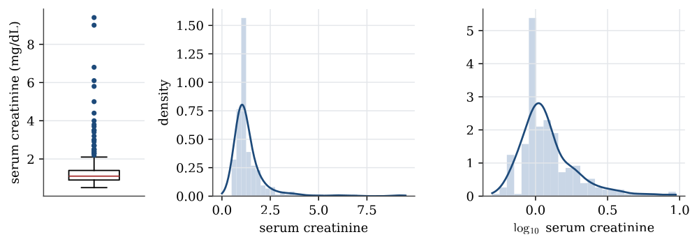
summary(heart$serum_creatinine)
#  Min. 1st Qu. Median   Mean 3rd Qu.   Max.
#  0.50    0.90   1.10   1.39    1.40   9.40
The mean is pulled above the median by a long right tail: the largest value, 9.4, is more than six times the median. The interquartile range is 1.4-0.9=0.5, so the upper whisker stops at the largest value below 1.4+1.5\times0.5=2.15, and 29 patients lie beyond it.
A histogram counts the data in a set of bins and draws a bar for each; its look depends on the choice of bins. A kernel density estimate smooths the data instead, placing a small bump at each observation and adding them up; its look depends on the width of the bumps, the bandwidth. Both show the same thing here: most patients near 1 mg/dL and a thin tail stretching to 9.
Transformations
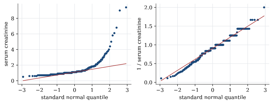
Strongly skewed data are often easier to summarise, and to model, after a transformation. A logarithm turns ratios into differences, so it spreads out the bunched values near zero and draws in the far tail. For serum creatinine the skewness, a measure of asymmetry that is zero for symmetric data, falls from 4.4 to 1.6 on the log scale. The reciprocal, 1/x, brings it to about zero. Transformations do not change the data, only the scale they are viewed on; the order of the patients stays the same, so the median of the transformed data is the transform of the median.
Definition 5 (Normal quantile plot) A normal quantile plot, or Q–Q plot, plots the sorted data against the quantiles of the standard normal distribution at the same fractions. If the data come from a normal distribution, the points lie close to a straight line, whose intercept and slope estimate the mean and standard deviation.
Curvature in a Q–Q plot is how a model check sees skewness. A right-skewed sample bends upwards at the right end; heavy tails bend away from the line at both ends.
One categorical and one quantitative variable
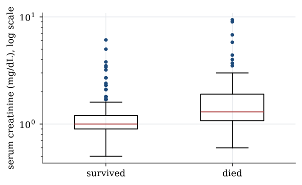
To compare a quantitative variable across groups, draw one boxplot or density per group on a common scale.
boxplot(serum_creatinine ~ death, data = heart, log = "y")The median serum creatinine is 1.0 mg/dL for patients who survived and 1.3 for those who died, and the means are 1.19 and 1.84. On the log scale the boxes overlap a good deal, but the whole distribution for those who died sits higher. High creatinine, a sign of poor kidney function, goes with death in this sample.
Two quantitative variables
Two quantitative variables are plotted against each other in a scatterplot, and their linear association is summarised by the sample correlation coefficient.
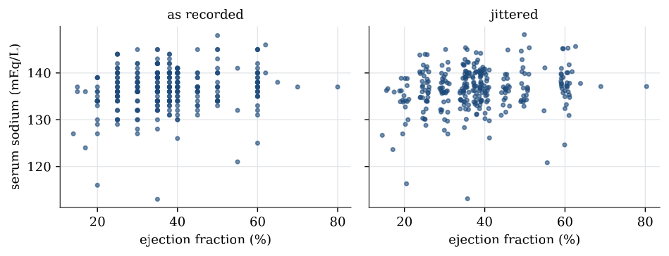
The ejection fraction was recorded in steps of 5 percentage points or so, with only 17 distinct values, and serum sodium as whole numbers. Many patients therefore share exactly the same point, and a plain scatterplot hides how many. Jittering, adding a small random amount to each coordinate before plotting, separates them; it changes the picture, not the data.
plot(jitter(serum_sodium) ~ jitter(ejection_fraction), data = heart)
cor(heart$serum_sodium, heart$ejection_fraction)   # 0.176
The correlation is 0.18: a weak tendency for patients with a higher ejection fraction to have more sodium. A correlation measures only linear association, and only in this sample; it does not say that one causes the other. Among the six quantitative measurements the largest correlation in absolute value is 0.19, between serum creatinine and sodium, so no pair moves strongly together.
Match the summary to the variable. Counts for categories, a centre and a spread for numbers, a scatterplot before a correlation. None of these is a conclusion about a parameter.
Questions on this topic
Open a question to attempt it. Its worked answer is folded away at the bottom of the page.
| Question | Answer |
|---|---|
| Classifying variables in a nutrition survey | ✓ |
| Reading a correlation | ✓ |
What links here
Pages (8)
- Statistical inference — via Descriptive statistics, quartile
- Studies, data, and evidence — via Descriptive statistics
- Using R — via Descriptive statistics, sample standard deviation
- Estimation examples — via normal quantile plot, sample variances
- Analysis of variance examples — via normal quantile plot
- Regression examples — via five-number summary, quartiles, normal quantile plot
- Linear model examples — via normal quantile plot
- Introduction to generalised linear models — via Descriptive statistics
Questions and answers (4)