Linear model examples
Part of Data analysis · 2 questions on this topic · What links here
Linear model examples
| Part | Data analysis |
| Chapter | 8 of 9 in this part |
| Previous | Regression examples |
| Next | Chi-squared examples |
| Questions | 2 |
| Definitions | Dummy variable coding |
| Figures | 2 |
Simple regression, multiple regression and the analysis of variance are all one model, the normal linear model. Seeing them that way explains why R fits all of them with lm, and how a categorical variable enters a regression. This page writes the design matrices out, fits a model that mixes quantitative and categorical explanatory variables, adds an interaction, and checks the result.
One model, many designs
In a normal linear model the response vector \mathbf Y=(Y_1,\ldots,Y_n)^{\mathsf T} is
\mathbf Y=X\boldsymbol\beta+\boldsymbol\varepsilon,\qquad \varepsilon_i\ \text{independent}\ \operatorname{N}(0,\sigma^2),
where the design matrix X holds the explanatory variables and \boldsymbol\beta the parameters. The least-squares estimate is \widehat{\boldsymbol\beta}=(X^{\mathsf T}X)^{-1}X^{\mathsf T}\mathbf Y; the geometry is in Bayesian linear regression.
For simple linear regression the design matrix has a column of ones and a column of x values:
X=\begin{pmatrix}1&x_1\\1&x_2\\\vdots&\vdots\\1&x_n\end{pmatrix},\qquad \boldsymbol\beta=\begin{pmatrix}\beta_0\\\beta_1\end{pmatrix}.
For a one-factor analysis of variance with three levels, R uses the first level as a baseline and adds an indicator column for each other level. With two observations per level, in level order,
X=\begin{pmatrix}1&0&0\\1&0&0\\1&1&0\\1&1&0\\1&0&1\\1&0&1\end{pmatrix},\qquad \boldsymbol\beta=\begin{pmatrix}\mu_1\\\mu_2-\mu_1\\\mu_3-\mu_1\end{pmatrix}.
Definition 1 (Dummy variable coding) A categorical explanatory variable with d levels enters a linear model through d-1 indicator columns, one for each level except a reference level. The coefficient of an indicator is the difference in mean response between that level and the reference level, with the other explanatory variables held fixed.
Using all d indicators together with the intercept would make the columns of X linearly dependent, since the indicators add up to the column of ones, and the parameters would not be identifiable. Dropping one level, the reference, removes the dependence. In R, a variable stored as numbers must be declared a factor, with factor(), or it will be fitted as a straight-line trend in its codes.
Birth weight
The birthwt data, in R’s MASS package, record 189 births. The response is the baby’s birth weight in grams; the explanatory variables include the mother’s age, her weight in pounds at her last menstrual period, her race (1 white, 2 black, 3 other), whether she smoked during pregnancy, and her history of hypertension and of uterine irritability.
Example 1 (Explaining birth weight) Question. Fit birth weight on the mother’s weight, age, race and smoking, and interpret each coefficient.
Solution.
library(MASS)
model1 <- lm(bwt ~ lwt + age + factor(race) + smoke, data = birthwt)
summary(model1)
#                Estimate Std. Error t value Pr(>|t|)
# (Intercept)    2839.433    321.435   8.834  8.2e-16 ***
# lwt               4.000      1.738   2.301  0.02249 *
# age              -1.948      9.820  -0.198  0.84299
# factor(race)2  -510.501    157.077  -3.250  0.00137 **
# factor(race)3  -398.644    119.579  -3.334  0.00104 **
# smoke          -401.720    109.241  -3.677  0.00031 ***
# Residual standard error: 682.1 on 183 degrees of freedom
# Multiple R-squared:  0.1483,  Adjusted R-squared:  0.125
# F-statistic: 6.373 on 5 and 183 DF,  p-value: 1.758e-05
The overall F test, p=1.8\times10^{-5}, says at least one of the variables is associated with birth weight. Taking them one at a time, each with the others held fixed:
- each extra pound of the mother’s weight goes with 4.0 g more birth weight on average (p=0.022);
- the mother’s age adds nothing once the other variables are known (p=0.84);
- babies of black mothers weigh 511 g less on average than those of white mothers, the reference level, and those of mothers of other races 399 g less (p=0.001 for both);
- babies of mothers who smoked weigh 402 g less than those of non-smokers of the same weight, age and race (p=0.0003).
The model explains only 15% of the variation in birth weight; the residual standard deviation is 682 g. These are observational data, so the coefficients are associations adjusted for the variables in the model, not effects: race, for instance, stands in for many unmeasured differences.
Interaction
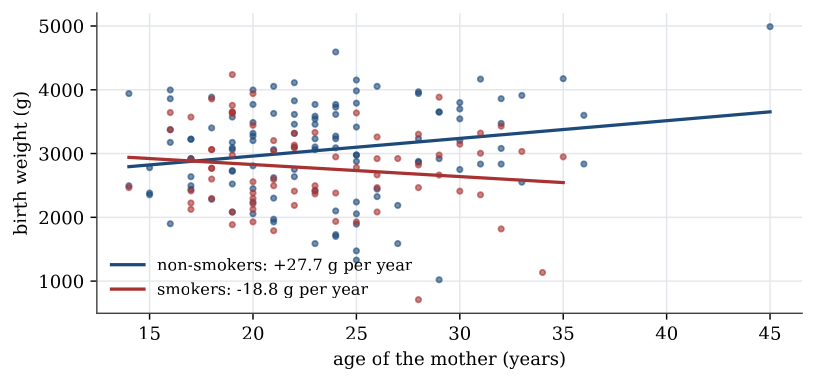
An interaction between a quantitative and a categorical variable lets the slope differ between groups. The model
\mathrm{bwt}=\beta_0+\beta_1\,\mathrm{age}+\beta_2\,\mathrm{smoke}+\beta_3\,\mathrm{age}\times\mathrm{smoke}+\varepsilon
has slope \beta_1 in age for non-smokers and \beta_1+\beta_3 for smokers.
Example 2 (Age and smoking interact) Question. Does the association between the mother’s age and birth weight depend on smoking?
Solution.
model2 <- lm(bwt ~ age * smoke, data = birthwt)
summary(model2)
#             Estimate Std. Error t value Pr(>|t|)
# (Intercept) 2406.058    292.190   8.235 3.18e-14 ***
# age           27.731     12.149   2.283   0.0236 *
# smoke        798.175    484.342   1.648   0.1011
# age:smoke    -46.572     20.447  -2.278   0.0239 *
The interaction is significant (p=0.024). For non-smokers, birth weight rises by 27.7 g per year of the mother’s age; for smokers, the slope is 27.73-46.57=-18.8 g per year, a decline. The coefficient of smoke alone, +798 g, is the difference between smokers and non-smokers at age zero, an extrapolation with no meaning; with an interaction in the model, main-effect coefficients have to be read together with it. Age had no association with birth weight in the additive model above precisely because the two groups’ slopes point in opposite directions and largely cancel.
Checking the final model
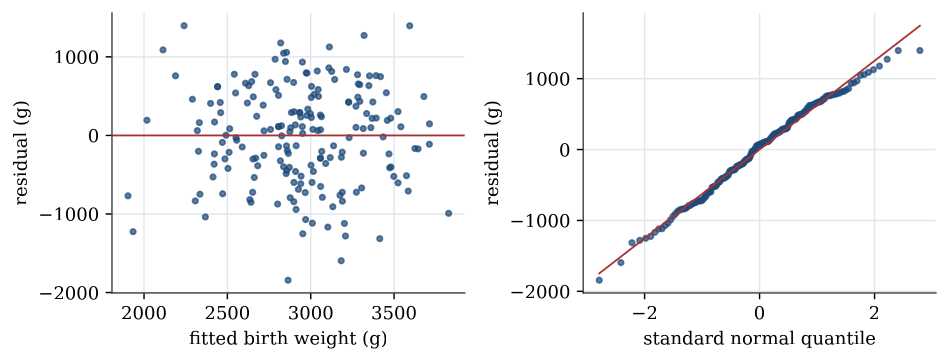
Adding uterine irritability and hypertension, and keeping the age–smoking interaction, gives the model
finalmodel <- lm(bwt ~ smoke + age + lwt + factor(race) + ui + ht + smoke:age,
                 data = birthwt)
plot(finalmodel, 1:2)
It explains 26% of the variation, with residual standard deviation 640 g; uterine irritability (-574 g) and hypertension (-599 g) both go with much lower birth weight. The residuals show no trend against the fitted values and roughly constant spread, and their normal quantile plot is close to a straight line, so the normal linear model is a reasonable description.
Transformations
When the residual plot curves or fans out, a transformation of the response or of an explanatory variable often straightens the relationship and steadies the variance. Common choices are \log y for a response whose spread grows with its mean, \sqrt y for counts, and \log x for an explanatory variable spanning several orders of magnitude. A model for \log y describes multiplicative effects: a unit increase in x multiplies the median of the response by e^\beta, roughly 1+\beta for small \beta. The residual plots are read on the scale that was fitted. Predictions are made on the transformed scale and then transformed back. The melanoma data in Linear regression are an example.
Regression and analysis of variance are the same linear model with different design matrices. A factor enters through indicator columns measured against a reference level; an interaction lets one variable’s slope depend on another; and every coefficient is read with the other variables held fixed.
Questions on this topic
Open a question to attempt it. Its worked answer is folded away at the bottom of the page.
| Question | Answer |
|---|---|
| How far sharks swim | ✓ |
| Wages, class, and gender | ✓ |
What links here
Pages (3)
- Using R — via Linear model examples
- Regression examples — via linear model
- Introduction to generalised linear models — via Linear model examples
See also
- Articles from this chapter: Dummy variable coding
- All data analysis chapters
- Glossary and index
- Distribution sheet and formula lookup