Multiple linear regression
Definition taught in Regression examples, part of Data analysis
Multiple linear regression
| Type | Definition |
| Taught in | Regression examples |
| Part | Data analysis |
| Worked examples | 2 |
The multiple linear regression model for a response Y and explanatory variables x_1,\ldots,x_p is
Y_i=\beta_0+\beta_1x_{i1}+\cdots+\beta_px_{ip}+\varepsilon_i,\qquad\varepsilon_i\ \text{independent}\ \operatorname{N}(0,\sigma^2),
with the \beta_j estimated by least squares. The coefficient \beta_j is the change in mean response for a unit increase in x_j with the other explanatory variables held fixed.
Examples
Height, shoe size and weight
Worked example from Regression examples
Question. Add weight to the regression of height on shoe size, and interpret both coefficients.
Solution.
model2 <- lm(height ~ shoe + weight, data = survey)
summary(model2)
#             Estimate Std. Error t value Pr(>|t|)
# (Intercept) 132.2677     5.2473  25.207  < 2e-16 ***
# shoe          0.5304     0.1962   2.703   0.0081 **
# weight        0.3744     0.0572   6.546 2.82e-09 ***
# Residual standard error: 7.785 on 97 degrees of freedom
# Multiple R-squared:  0.4301,  Adjusted R-squared:  0.4184
# F-statistic: 36.61 on 2 and 97 DF,  p-value: 1.429e-12
confint(model2)
#                   2.5 %      97.5 %
# (Intercept) 121.8533072 142.6821199
# shoe          0.1410087   0.9198251
# weight        0.2608887   0.4879514
Among students of the same weight, one more centimetre of shoe goes with 0.53 cm more height on average (p=0.008); among students with the same shoe size, one more kilogram goes with 0.37 cm more height (p=3\times10^{-9}). The shoe-size coefficient has roughly halved from the simple regression, because shoe size and weight are themselves related: part of what shoe size “explained” alone is now credited to weight. Together the two variables account for 43% of the variation in height, up from 18%, and the residual standard error falls from 9.3 to 7.8 cm. The adjusted R^2, 0.418, is barely below R^2, so the gain is not an artefact of adding a parameter.
For a student with shoe size 30 cm and weight 75 kg, predict(model2, data.frame(shoe = 30, weight = 75), interval = "conf") gives a mean height of 132.27+0.5304\times30+0.3744\times75=176.3 cm, with 95% interval (174.2,\ 178.4).
Explaining birth weight
Worked example from Linear model examples
Question. Fit birth weight on the mother’s weight, age, race and smoking, and interpret each coefficient.
Solution.
library(MASS)
model1 <- lm(bwt ~ lwt + age + factor(race) + smoke, data = birthwt)
summary(model1)
#                Estimate Std. Error t value Pr(>|t|)
# (Intercept)    2839.433    321.435   8.834  8.2e-16 ***
# lwt               4.000      1.738   2.301  0.02249 *
# age              -1.948      9.820  -0.198  0.84299
# factor(race)2  -510.501    157.077  -3.250  0.00137 **
# factor(race)3  -398.644    119.579  -3.334  0.00104 **
# smoke          -401.720    109.241  -3.677  0.00031 ***
# Residual standard error: 682.1 on 183 degrees of freedom
# Multiple R-squared:  0.1483,  Adjusted R-squared:  0.125
# F-statistic: 6.373 on 5 and 183 DF,  p-value: 1.758e-05
The overall F test, p=1.8\times10^{-5}, says at least one of the variables is associated with birth weight. Taking them one at a time, each with the others held fixed:
- each extra pound of the mother’s weight goes with 4.0 g more birth weight on average (p=0.022);
- the mother’s age adds nothing once the other variables are known (p=0.84);
- babies of black mothers weigh 511 g less on average than those of white mothers, the reference level, and those of mothers of other races 399 g less (p=0.001 for both);
- babies of mothers who smoked weigh 402 g less than those of non-smokers of the same weight, age and race (p=0.0003).
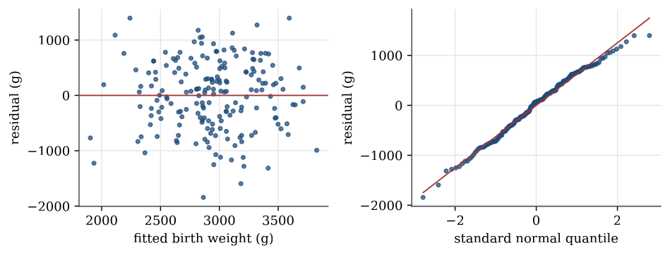
The model explains only 15% of the variation in birth weight; the residual standard deviation is 682 g. These are observational data, so the coefficients are associations adjusted for the variables in the model, not effects: race, for instance, stands in for many unmeasured differences.
Figures
Used in
- Taught in Regression examples, where the derivation and examples are.
- Also used in Linear model examples
- All 3 questions on Regression examples