Marginal models, and two responses at once
Part of Correlated data · 6 questions on this topic · What links here
Marginal models, and two responses at once
| Part | Correlated data |
| Chapter | 3 of 4 in this part |
| Previous | Random slopes, and a binary mixed model |
| Next | Three species on one hillside |
| Questions | 6 |
| Definitions | Marginal model |
| Figures | 2 |
A mixed model explains the correlation: a shared intercept, a shared slope, something that can be simulated. A marginal model does not. It describes the average curve in the population and then corrects the standard errors for whatever dependence is left. This chapter is that second description, first for one response measured repeatedly, then for two different responses on the same person.
The average, and the person
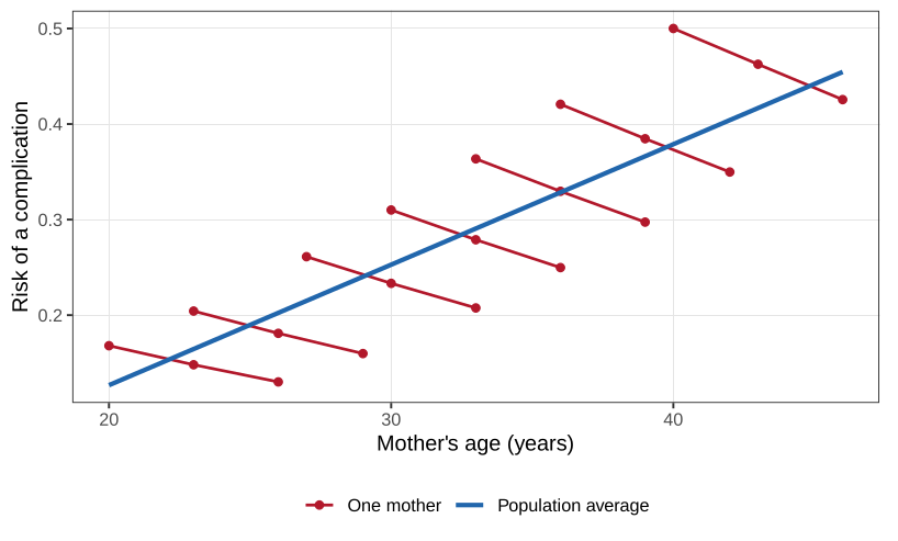
Plot risk of a birth complication against the mother’s age and the cloud rises. Label the points by mother and the story reverses.
Within a mother, the second and third births are a little safer than the first, even though she is older. The red lines in Figure 1, one intercept and one slope per mother, are the subject-specific model of the previous chapter. The blue line through the whole cloud is the marginal, or population-average, model. They answer different questions. “What happens to this woman as she ages?” is the red line. “What does the risk look like, in this population, at a given age?” is the blue one. Which random-effects model is placed inside each mother can change the red slopes. The blue slope is the average association, and it does not have to move when the working correlation changes.
That is the attraction. We specify a mean that has an interpretation as a population average, a variance that depends on that mean, and a working association within each cluster. The working association does not have to be right. After the fit, a sandwich estimator replaces the model-based variance of \hat{\boldsymbol{\beta}} by one that uses the empirical residuals. If the mean is correctly specified, \hat{\boldsymbol{\beta}} is consistent, and so is the sandwich variance, even when the working correlation is wrong. The rate depends on how wrong it was. The guarantee is asymptotic in the number of clusters and, in the theory, in the size of each cluster. A handful of clusters, or one cluster with almost all the data, is not a setting in which the robust column should be trusted blindly.
For two binary variables the correlation cannot be chosen freely. A coin with success probability 0.2 and a coin with success probability 0.8 cannot be perfectly correlated. The largest correlation they can have is 0.25. A correlation is the wrong primitive once the margins are not normal. An odds ratio, or some other association that is free of that constraint, is the working model. And a mean plus a covariance does not determine a joint Poisson distribution. There is no unique bivariate Poisson. The marginal model does not need one.
Definition 1 A marginal model for clustered responses has three parts.
- A mean, g(\mathrm{E}(Y_{ji}\mid {\boldsymbol{X}}_{ji}))={\boldsymbol{X}}_{ji}^\top\boldsymbol{\beta}, the same link and the same linear predictor as for independent data.
- A variance, \mathrm{Var}(Y_{ji}\mid {\boldsymbol{X}}_{ji})=\phi V(\mu_{ji}), depending on the covariates only through the mean.
- A working association within a cluster, allowed to depend on the two means and on further association parameters.
The estimator solves the generalised estimating equations, the dependent version of the quasi-score. Liang and Zeger (1986) showed that the fit does not require integrating up to a likelihood. If the working variance happens to equal the truth, the sandwich collapses to the model-based inverse information, which is the best variance available. If it does not, the variance of \hat{\boldsymbol{\beta}} is the sandwich: model-based bread on the outside, the empirical residual covariance in the middle. Packages still call those pieces bread and meat.
Warp breaks
Yarn was spun at two factories, at low, medium, and high tension, and the number of breaks in a fixed length was recorded, nine replicates of each tension at each factory. Breaks are a count. Yarn from the same factory shares machines, material, and a standard, so the factory is the cluster. Two clusters is a small number for a sandwich. The model is still fitted. The robust column is the one the theory prefers, and it is not a precise standard error from a large number of factories.
An exchangeable working correlation says every pair of looms from the same factory has the same correlation. With a Poisson mean and a log link,
need <- function(pkg) {
  if (!requireNamespace(pkg, quietly = TRUE)) {
    install.packages(pkg, repos = "https://cloud.r-project.org")
  }
  suppressPackageStartupMessages(library(pkg, character.only = TRUE))
}
need("gee")
data(warpbreaks)
warpbreaks$factory <- warpbreaks$wool
warpbreaks <- warpbreaks[order(warpbreaks$factory), ]
exchangeable <- gee(breaks ~ tension, id = factory, data = warpbreaks,
                    family = poisson, corstr = "exchangeable")
summary(exchangeable)
ar1 <- gee(breaks ~ tension, id = factory, data = warpbreaks,
           family = poisson, corstr = "AR-M", Mv = 1)
summary(ar1)
ar1$working.correlation[1:4, 1:4]
gaussian_ar <- gee(breaks ~ tension, id = factory, data = warpbreaks,
                   family = gaussian(link = "log"), corstr = "AR-M", Mv = 1)
summary(gaussian_ar)
Estimate Naive SE Robust SE
(Intercept) 3.594 0.091 0.159
tensionM -0.321 0.128 0.223
tensionH -0.518 0.136 0.064The scale estimate is 4.60, far from 1: these counts are more variable than a Poisson. The working correlation is about 0.021. Low tension, the baseline, has fitted mean \exp(3.594)\approx 36 breaks. Medium tension multiplies that mean by \exp(-0.321)=0.73. High tension multiplies it by \exp(-0.518)=0.60. On the naive standard errors, medium tension is detected (z=-2.51). On the robust standard errors it is not (z=-1.44). High tension is detected either way, and the robust standard error is about half the naive one. The two columns disagree, which is evidence that the Poisson variance and the exchangeable correlation are not the truth. The robust column is the one that remains consistent if the mean is right.
The looms were recorded in the order they came off the machine. Then exchangeable correlation is the wrong working model. An AR(1) working correlation sets \mathrm{Corr}(Y_t,Y_{t+k})=\gamma^{|k|}. The lag-1 value is 0.041, then 0.041^2 at lag 2 and 0.041^3 at lag 3. The coefficients barely move: intercept 3.595, medium -0.325, high -0.518. The naive standard errors move, because the working model moved. The robust standard errors stay where they were, to two decimals. That is the theorem, visible in one table. A third fit keeps the log mean and the AR(1) working correlation, and replaces the Poisson variance by a constant variance, a Gaussian family with a log link. A constant-variance model for counts is a poor variance story. The coefficients are again 3.595, -0.324, -0.518, and the robust standard errors again match the previous robust column. The scale estimate, 141, is a variance on the count scale and is not a quantity to interpret as a Poisson dispersion.
If the mean is the right function of the covariates, the estimates of \boldsymbol{\beta} and the sandwich standard errors settle in the same place whatever working correlation the fit starts from. The naive standard errors move. A large gap between the two columns means the working variance was wrong. It does not, by itself, mean the robust column is wrong.
The gap here is large for every working model fitted above, so none of them is close to the true covariance. The robust standard errors are still the ones the asymptotic result licenses. They are not a substitute for having more than two factories.
Two responses, one person
A longitudinal study repeats the same measurement. A vector regression measures different things on the same unit, and each margin can have its own link and its own variance. Height and arm span, or burn area and death, are not repeated measures of one variable. Write component k on unit i as \mathrm{E}(Y_{ik}\mid {\boldsymbol{X}}_{ik})=\mu_k({\boldsymbol{X}}_{ik}^\top\boldsymbol{\beta}_k), \qquad \mathrm{Var}(Y_{ik}\mid {\boldsymbol{X}}_{ik})=\phi_k V_k(\mu_{ik}). The \boldsymbol{\beta}_k are different parameters. A working association across components can be wrong, and the sandwich corrects it afterwards.
Fan and Gibbon’s burn data, as quoted by Song, have two responses of equal interest on each patient: the log of burn area plus one, a continuous severity, and an indicator of death. Age is the covariate. The margins, fitted independently, are \widehat{\mathrm{E}}(\text{severity}\mid \text{age})=6.7118+0.0035\,\text{age}, \widehat{\mathrm{P}}(\text{death}\mid \text{age}) =\frac{\exp(-3.6891+0.0508\,\text{age})}{1+\exp(-3.6891+0.0508\,\text{age})}. The sandwich standard errors of the two slopes are 0.0017 and 0.0051. The ratios are 0.0035/0.0017=2.1, \qquad 0.0508/0.0051=10.0. Age is associated with worse burns and with a higher chance of death. The direction is not the one a purely biological story about fragile infants would have suggested. Older children are the ones who get far enough into a kitchen, or a fire, to be burned this badly. The association is marginal and confounded with exposure.
The working model here was independence: two separate glm fits, stacked. The sandwich uses the cross-products of the two residuals on the same child, so the reported standard errors are not the independence standard errors.
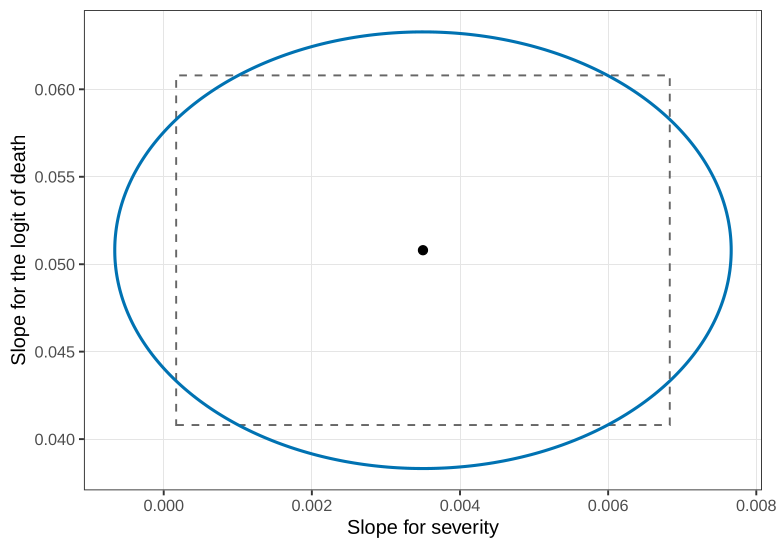
A joint confidence region for the two slopes is an ellipse, as in Figure 2, not the rectangle obtained by crossing the two marginal intervals. A pair that is acceptable one slope at a time can sit outside the ellipse. The ellipse puts more of its mass on “age matters for both” and less on “age matters strongly for severity and not at all for death”.
A genuine bivariate Poisson, when a distribution is wanted rather than a working covariance, is usually built by sharing a third Poisson: X_1=Y_1+Y_2, X_2=Y_2+Y_3, with Y_1,Y_2,Y_3 independent Poissons. The margins are Poisson and the correlation is positive. A minus sign can produce a negative correlation and can also produce a negative count, which is not a Poisson margin. The estimating-equation model simply declares two Poisson margins and a correlation in (-1,1), and does not claim that a joint distribution with those moments exists. That is the same descriptive licence as a quasi-likelihood.
The three plant species at a set of altitudes, where the association is an odds ratio rather than a correlation of two different kinds of measurement, are the next chapter.
From the exchangeable warp-break fit, compute \exp(3.594), \exp(-0.321) and \exp(-0.518), and state them as a baseline mean and two multiplicative comparisons with low tension.
Explain why the robust z-statistic for medium tension changes the conclusion that the naive z-statistic gave, and why the coefficients themselves did not have to move when the working correlation changed from exchangeable to AR(1).
The burn-severity slope is 0.0035 with sandwich standard error 0.0017. Compute the z-statistic and say what “marginal” means for that slope.
Why can two Bernoulli random variables with means 0.2 and 0.8 not have correlation 1?
Questions on this topic
Open a question to attempt it. Its worked answer is folded away at the bottom of the page.
What links here
Pages (2)
- Random slopes, and a binary mixed model — via Marginal models
- Three species on one hillside — via sandwich standard errors
Questions and answers (5)
- Question 20 (answer) · C38 · C39 · C40 · C41
See also
- Articles from this chapter: Marginal model
- All correlated data chapters
- Glossary and index
- Distribution sheet and formula lookup