Functions of random variables and limit theorems
Part of Probability · 21 questions on this topic · What links here
Functions of random variables and limit theorems
| Part | Probability |
| Chapter | 5 of 7 in this part |
| Previous | Joint distributions |
| Next | Markov chains |
| Questions | 21 |
| Definitions | Multivariate normal distribution · Normal linear model |
| Results | Transformation rule · Affine images of normal vectors · Law of large numbers · Central limit theorem |
| Figures | 2 |
A function of a random variable is another random variable. Its distribution can be read off the original distribution by inverting the function, by a linear change of variables, or by the Jacobian formula in several dimensions. The same calculus gives the joint normal family and the normal linear model. Limit theorems say what happens to an average as the number of terms grows: it settles on the mean, and the fluctuations around the mean become normal.
The one-dimensional families used here are on the common distributions page. Generating a variable by inverting its distribution function is the inverse-transform method. Estimation for the normal linear model, including the least-squares geometry and the posterior, is on Bayesian linear regression. This chapter stops at the probability model.
One variable, and a sum
Let X be continuous with density f_X, and let Y=g(X) with g strictly monotone and differentiable. Then
f_Y(y)=f_X\bigl(g^{-1}(y)\bigr)\,\bigl|\tfrac{d}{dy}g^{-1}(y)\bigr|.
An affine map Y=aX+b with a\ne 0 is the case everyone uses: f_Y(y)=f_X((y-b)/a)/|a|. If X is standard normal and Y=1+2X, then Y\sim\operatorname{N}(1,4). If X\sim\operatorname{Exp}(\lambda) and Y=1+2X, the same formula shifts and stretches the exponential density.
The square of a standard normal variable is chi-squared with one degree of freedom, which is the gamma law with shape 1/2 and rate 1/2. The distribution function of Y=X^2 is \mathbb{P}(-\sqrt{y}\le X\le\sqrt{y}) for y>0, and differentiating produces the density.
Example 1 (The square of a standard normal) Let X\sim\operatorname{N}(0,1) and Y=X^2.
Question. Find the density of Y.
Solution. The map x\mapsto x^2 is not monotone, so work with the distribution function. For y>0,
F_Y(y)=\mathbb{P}(-\sqrt y\le X\le\sqrt y)=\Phi(\sqrt y)-\Phi(-\sqrt y)=2\Phi(\sqrt y)-1.
Differentiating, with \Phi'=\varphi the standard normal density,
f_Y(y)=2\varphi(\sqrt y)\cdot\frac1{2\sqrt y}=\frac{1}{\sqrt{2\pi}}\,y^{-1/2}e^{-y/2},\qquad y>0.
That is the \operatorname{Gamma}(1/2,1/2) density, the chi-squared law with one degree of freedom, since \Gamma(1/2)=\sqrt\pi.
For a maximum or a minimum the distribution function is easier than the density. If X_1,\ldots,X_n are independent with distribution function F and survival function 1-F, then
\mathbb{P}(\max_i X_i\le x)=F(x)^n, \qquad \mathbb{P}(\min_i X_i>x)=(1-F(x))^n.
The density follows by differentiation. This is why the minimum of n independent exponential variables with rate \lambda is exponential with rate n\lambda.
Example 2 (A series of exponential components) A system has five components in series, so it fails as soon as one component fails. The components’ lifetimes are independent and exponential with mean 1000 hours.
Question. Find the distribution and the mean of the system lifetime.
Solution. The system lifetime is T=\min_iX_i. Each X_i has survival function e^{-x/1000}, so
\mathbb{P}(T>t)=\bigl(e^{-t/1000}\bigr)^5=e^{-t/200}.
T is exponential with rate 5/1000, and its mean is 200 hours. Five components in series fail five times as fast as one. The maximum, which is the lifetime of the same five components in parallel, has distribution function (1-e^{-t/1000})^5 and is not exponential.
The sum of two independent continuous variables has density equal to the convolution
f_{X+Y}(z)=\int_{-\infty}^{\infty} f_X(x)\,f_Y(z-x)\,\,\mathrm{d} x.
Two independent uniform variables on [0,1] have a triangular sum: the density of the sum is z on (0,1) and 2-z on (1,2). The moment generating function is usually faster when the sum stays in a named family. Independent gamma variables with the same rate were added that way in Joint distributions.
Example 3 (The sum of two uniforms) Let X and Y be independent and uniform on [0,1], and Z=X+Y.
Question. Find the density of Z.
Solution. By the convolution formula, f_Z(z)=\int f_X(x)f_Y(z-x)\,\mathrm{d} x. The integrand is 1 when both 0\le x\le1 and 0\le z-x\le1, that is when \max(0,z-1)\le x\le\min(1,z), and 0 otherwise. The length of that interval is z for 0\le z\le1 and 2-z for 1\le z\le2, so
f_Z(z)=\begin{cases}z,&0\le z\le1,\\ 2-z,&1\le z\le2.\end{cases}
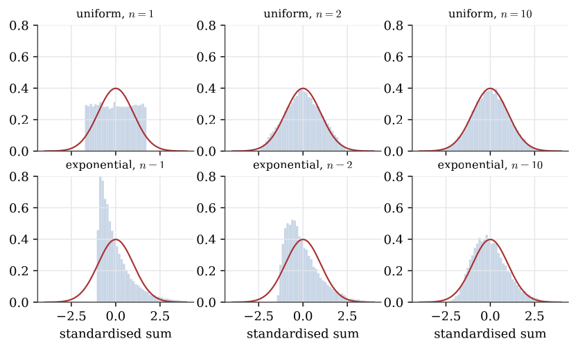
The sum of two flat densities is a triangle. Adding more uniforms rounds the shape off further, towards the normal curve of the central limit theorem below.
The transformation rule
Theorem 1 (Transformation rule) Let \mathbf{X} take values in an open set of \mathbb{R}^n with density f_{\mathbf{X}}, and let \mathbf{Z}=g(\mathbf{X}) where g is a smooth bijection onto its image, with inverse g^{-1} and Jacobian determinant J that does not vanish. The density of \mathbf{Z} is
f_{\mathbf{Z}}(\mathbf{z})=f_{\mathbf{X}}\bigl(g^{-1}(\mathbf{z})\bigr)\,\bigl|\det Dg^{-1}(\mathbf{z})\bigr|.
Equivalently, if the Jacobian is computed for g rather than for the inverse, divide by |\det Dg| evaluated at the preimage. For a linear map \mathbf{Z}=A\mathbf{X} with A invertible, f_{\mathbf{Z}}(\mathbf{z})=f_{\mathbf{X}}(A^{-1}\mathbf{z})/|\det A|.
The absolute value of the Jacobian is the local change in volume. Probability in a small region is density times volume, so the density must be divided by that factor.
Box–Muller is this rule in the plane. Let U,V be independent and uniform on (0,1), and set
Z_1=\sqrt{-2\log U}\,\cos(2\pi V), \qquad Z_2=\sqrt{-2\log U}\,\sin(2\pi V).
Passing to polar-type coordinates and computing the Jacobian shows that (Z_1,Z_2) has joint density (2\pi)^{-1}\exp(-(z_1^2+z_2^2)/2) on \mathbb{R}^2, the product of two standard normal densities. The construction is the one used in Simulation when a normal generator has to be built from uniforms.
A second standard example splits a pair of independent exponential variables. Let X and Y be independent and exponential with rate 1, and set U=X+Y and V=X/(X+Y). The map (u,v)\mapsto(uv,\,u(1-v)) has Jacobian determinant of absolute value u. The joint density of (U,V) is u e^{-u} on u>0, 0<v<1, which factors into a \operatorname{Gamma}(2,1) density for U and a uniform density for V. So U and V are independent.
Jointly normal variables
Definition 1 (Multivariate normal distribution) A random vector \mathbf{Z} in \mathbb{R}^n is multivariate normal with mean \boldsymbol\mu and covariance matrix \Sigma, when \Sigma is positive definite and the density is
f(\mathbf{z})=(2\pi)^{-n/2}\,|\Sigma|^{-1/2}\,\exp\Bigl(-\tfrac12(\mathbf{z}-\boldsymbol\mu)^\top\Sigma^{-1}(\mathbf{z}-\boldsymbol\mu)\Bigr).
If \mathbf{X} has independent standard normal coordinates and \Sigma=BB^\top, then \boldsymbol\mu+B\mathbf{X} has this distribution. The representation is the definition used when \Sigma is only positive semidefinite and no density exists.
In two dimensions, with means \mu_1,\mu_2, variances \sigma_1^2,\sigma_2^2 and correlation \rho, the density has level sets that are ellipses tilted by \rho. The case \rho=0 is independence. That is special to the normal family: for jointly normal coordinates, zero covariance is independence, because the quadratic form in the exponent then splits into a sum.
Theorem 2 (Affine images of normal vectors) If X_i\sim\operatorname{N}(\mu_i,\sigma_i^2) are independent and a,b_1,\ldots,b_n are constants, then
a+\sum_{i=1}^n b_i X_i \sim \operatorname{N}\Bigl(a+\sum_{i=1}^n b_i\mu_i,\;\sum_{i=1}^n b_i^2\sigma_i^2\Bigr).
The same conclusion holds for a jointly normal vector and any affine image, with the output variance \mathbf{b}^\top\Sigma\mathbf{b}.
A machine that produces diameters X\sim\operatorname{N}(1,0.01) and then records a+bX is still producing a normal measurement. The mean and variance are the only things the affine map can change.
Example 4 (Ball bearings and a sieve) Ball bearings have diameters X\sim\operatorname{N}(1,0.01) cm. They are dropped through a sieve whose holes have diameters Y\sim\operatorname{N}(1.1,0.04) cm, independent of the balls.
Question. What is the probability that a ball falls through a hole?
Solution. The ball falls through when Y>X. Because X and Y are independent normals, Y-X is normal with mean 1.1-1=0.1 and variance 0.04+0.01=0.05. So
\mathbb{P}(Y-X>0)=\mathbb{P}\Bigl(Z>\frac{-0.1}{\sqrt{0.05}}\Bigr)=\Phi(0.447)=0.67.
The variances add even though the variable is a difference.
The normal linear model
Definition 2 (Normal linear model) A normal linear model for a response vector \mathbf{Y}\in\mathbb{R}^n says
\mathbf{Y}=A\boldsymbol\beta+\boldsymbol\varepsilon, \qquad \boldsymbol\varepsilon\sim\operatorname{N}(\mathbf{0},\,\sigma^2 I_n),
with A a known n\times p matrix of full column rank, \boldsymbol\beta\in\mathbb{R}^p an unknown coefficient vector, and \sigma^2>0.
The coordinates of \mathbf{Y} are independent and normal. The ith coordinate has mean equal to the ith row of A times \boldsymbol\beta, and every coordinate has variance \sigma^2. The multiple linear regression model is the case in which the ith row of A is (1, x_{i1},\ldots,x_{i,p-1}), so the mean is an intercept plus a linear function of the covariates.
This is a probability statement about \mathbf{Y} once \boldsymbol\beta and \sigma^2 are fixed. It is not yet an estimate of \boldsymbol\beta. Fitting, the geometry of least squares, and the posterior under a prior on (\boldsymbol\beta,\sigma^2) are developed on Bayesian linear regression.
Limit theorems
Let X_1,X_2,\ldots be independent, identically distributed, with \mathbb{E} X_i=\mu, and write S_n=X_1+\cdots+X_n.
Theorem 3 (Law of large numbers) If the mean \mu exists, the strong law says
\mathbb{P}\Bigl(\lim_{n\to\infty} S_n/n=\mu\Bigr)=1.
If in addition the variance is finite, the weak law says that for every \varepsilon>0,
\lim_{n\to\infty}\mathbb{P}\bigl(|S_n/n-\mu|>\varepsilon\bigr)=0.
The weak law under a finite variance follows from Chebyshev’s inequality: \mathbb{P}(|S_n/n-\mu|>\varepsilon)\le \operatorname{Var}(S_n/n)/\varepsilon^2=\operatorname{Var}(X_1)/(n\varepsilon^2), which tends to zero.
The sample average converges to the expectation. That is the justification for estimating an unknown mean by the average of repeated measurements, and for reading a long-run relative frequency as a probability. The weak law says the probability of a large error disappears. The strong law says the error itself disappears, except on a set of outcomes of probability zero.
Chebyshev’s inequality, used above, is the general bound \mathbb{P}(|X-\mathbb{E} X|\ge \varepsilon)\le \operatorname{Var}(X)/\varepsilon^2, and Markov’s inequality is \mathbb{P}(X\ge x)\le \mathbb{E} X/x for a non-negative X and x>0.
Theorem 4 (Central limit theorem) If the X_i are independent and identically distributed with mean \mu and variance \sigma^2\in(0,\infty), then for every x
\lim_{n\to\infty}\mathbb{P}\Bigl(\frac{S_n-n\mu}{\sigma\sqrt{n}}\le x\Bigr)=\Phi(x),
where \Phi is the standard normal distribution function.
The shape of the parent distribution washes out of the centred and scaled sum. What remains is the standard normal distribution. For large n, S_n is approximately \operatorname{N}(n\mu, n\sigma^2), and the sample average is approximately \operatorname{N}(\mu,\sigma^2/n).
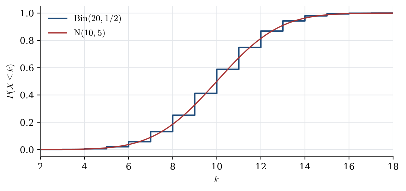
A binomial count X\sim\operatorname{Bin}(n,p) is a sum of n Bernoulli trials, so for large n
\mathbb{P}(X\le k)\approx \Phi\Bigl(\frac{k-np}{\sqrt{np(1-p)}}\Bigr).
Example 5 (Normal approximation to a binomial) Let X\sim\operatorname{Bin}(20,1/2).
Question. Approximate \mathbb{P}(X\le8) by the central limit theorem, with and without a continuity correction, and compare with the exact value.
Solution. Here np=10 and np(1-p)=5. The exact probability is 0.2517. The plain approximation gives
\mathbb{P}(X\le8)\approx\Phi\Bigl(\frac{8-10}{\sqrt5}\Bigr)=\Phi(-0.894)=0.186,
which is poor. X is integer-valued, so \mathbb{P}(X\le8)=\mathbb{P}(X\le8.5), and the normal curve should be read at the midpoint between 8 and 9:
\mathbb{P}(X\le8)\approx\Phi\Bigl(\frac{8.5-10}{\sqrt5}\Bigr)=\Phi(-0.671)=0.251,
almost exact. A usual rule of thumb asks for both np and n(1-p) to be above 5.
The same approximation, applied to a sum of independent uniforms or to a sum of independent exponential variables, is how a probability about an average is evaluated when the exact distribution is awkward. The distribution function \Phi is the one attached to the normal law on the common distributions page.
Monotone maps change the density by the derivative of the inverse. Smooth maps in several dimensions change it by the absolute value of the Jacobian. Averages of independent copies converge to the mean, and the scaled fluctuation converges to a standard normal variable.
Questions on this topic
Open a question to attempt it. Its worked answer is folded away at the bottom of the page.
What links here
Pages (19)
- Random variables and distributions — via transformation rule, Functions of random variables and limit theorems
- Simulation — via Jacobian, Functions of random variables and limit theorems
- Joint distributions — via jointly normal, transformation rule
- Markov chains — via law of large numbers
- Statistical inference — via central limit theorem, law of large numbers, affine images of normal vectors
- Estimation — via law of large numbers
- Confidence intervals — via central limit theorem
- Hypothesis tests — via central limit theorem, continuity correction
- Chi-squared tests — via central limit theorem
- Linear regression — via Functions of random variables and limit theorems, jointly normal
- Estimation examples — via central limit theorem, continuity correction
- Testing examples — via central limit theorem
- Linear model examples — via normal linear model
- Chi-squared examples — via continuity correction
- Bayesian linear regression — via multivariate normal
- Introduction to generalised linear models — via central limit theorem
- Standard errors, and models for counts — via central limit theorem
- Random slopes, and a binary mixed model — via multivariate normal
- Dependence along a series — via multivariate normal
Questions and answers (17)
- A normal approximation on an interval (answer) · Sum and proportion of two exponentials · A sieve for blueberries (answer) · Ten successive exponential components · A Poisson mean (answer) · The correlation test is the slope test (answer) · A logit-normal prior for a coin (answer) · A bivariate-normal Gibbs sampler · Random-walk Metropolis for a correlated normal (answer) · Q25 (answer) · Q27 (answer) · Q28 (answer) · Q52 (answer) · Question 1 (answer) · Question 7 (answer) · Question 9 (answer) · C34 (answer)