Analysis of variance
Part of Statistical inference · 6 questions on this topic · What links here
Analysis of variance
| Part | Statistical inference |
| Chapter | 7 of 7 in this part |
| Previous | Linear regression |
| Questions | 6 |
| Definitions | One-way analysis of variance · Contrast · Tukey intervals · Randomised block design |
| Results | ANOVA sum of squares decomposition · ANOVA F distribution |
| Figures | 3 |
Analysis of variance compares several means by splitting the total sum of squares into a part between groups and a part within groups. With two groups the resulting F statistic is the square of the two-sample t statistic from Hypothesis tests. With a non-normal response the parallel comparison of fitted models is an analysis of deviance. The normal linear model underneath both is the one in Linear regression and, with a prior, in Bayesian linear regression. The F law is defined in Statistical inference.
Between and within
Four age groups of 10 people each do a physical test, and the increase in heart rate is recorded.
| Age 10–19 | Age 20–39 | Age 40–59 | Age 60–69 |
|---|---|---|---|
| 29 | 24 | 37 | 28 |
| 33 | 27 | 25 | 29 |
| 26 | 33 | 22 | 34 |
| 27 | 31 | 33 | 36 |
| 39 | 21 | 28 | 21 |
| 35 | 28 | 26 | 20 |
| 33 | 24 | 30 | 25 |
| 29 | 34 | 34 | 24 |
| 36 | 21 | 27 | 33 |
| 22 | 32 | 33 | 32 |
The group means are 30.9, 27.5, 29.5 and 28.2. Do the age groups differ in mean increase?
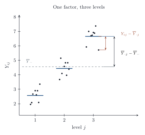
There is no four-sample t test. A t statistic compares two means through their difference, and four means have six differences, which are not independent. The way forward is to compare the variation of the group means about the grand mean with the variation of the observations inside each group. Here the spread within every group, about 4 to 5 beats, is much larger than the spread between the four means. That suggests the means are equal and age is not a factor that explains the increase.
One factor
Definition 1 (One-way analysis of variance) In a completely randomised one-factor design, responses at level j=1,\ldots,k follow
Y_{ij}=\mu_j+\varepsilon_{ij}, \qquad \varepsilon_{ij}\ \text{independent}\ \operatorname{N}(0,\sigma^2),
with n_j observations at level j and n=\sum_j n_j. The levels are the treatments. The hypothesis of equal means is H_0:\mu_1=\cdots=\mu_k.
The model is the k-sample version of the two-sample t model: k independent normal samples with a common variance. \mu_j is the true mean at level j, and \varepsilon_{ij} is the deviation of observation i from it. The model has k+1 unknown parameters. Write \overline Y_{\cdot j} for the mean at level j and \overline Y_{\cdot\cdot} for the grand mean of all n observations. The maximum likelihood estimators are
\widehat\mu_j=\overline Y_{\cdot j},\qquad \widehat\sigma^2=\frac1n\sum_{j=1}^k\sum_{i=1}^{n_j}(Y_{ij}-\overline Y_{\cdot j})^2,
by the same calculation as for one normal sample, done group by group with a shared variance. For the heart rates, \widehat\sigma^2=935.5/40=23.4.
Proposition 1 (ANOVA sum of squares decomposition) With
\mathrm{SS}_{\mathrm{total}}=\sum_{j=1}^k\sum_{i=1}^{n_j}(Y_{ij}-\overline Y_{\cdot\cdot})^2, \qquad \mathrm{SS}_{\mathrm{treatment}}=\sum_{j=1}^k n_j(\overline Y_{\cdot j}-\overline Y_{\cdot\cdot})^2, \qquad \mathrm{SS}_{\mathrm{error}}=\sum_{j=1}^k\sum_{i=1}^{n_j}(Y_{ij}-\overline Y_{\cdot j})^2,
the total sum of squares splits as \mathrm{SS}_{\mathrm{total}}=\mathrm{SS}_{\mathrm{treatment}}+\mathrm{SS}_{\mathrm{error}}.
Write each deviation from the grand mean as a deviation of the group mean plus a deviation within the group, Y_{ij}-\overline Y_{\cdot\cdot}=(\overline Y_{\cdot j}-\overline Y_{\cdot\cdot})+(Y_{ij}-\overline Y_{\cdot j}), and square. The cross term vanishes group by group,
\sum_{j=1}^k(\overline Y_{\cdot j}-\overline Y_{\cdot\cdot})\sum_{i=1}^{n_j}(Y_{ij}-\overline Y_{\cdot j})=0,
because deviations from a group mean sum to zero within that group. \mathrm{SS}_{\mathrm{treatment}} measures variation between the groups and \mathrm{SS}_{\mathrm{error}} measures variation within them.
Theorem 1 (ANOVA F distribution) In the one-way model, \mathrm{SS}_{\mathrm{error}}/\sigma^2 is \chi^2_{n-k}, and it is independent of \mathrm{SS}_{\mathrm{treatment}}. Under H_0:\mu_1=\cdots=\mu_k, \mathrm{SS}_{\mathrm{treatment}}/\sigma^2 is \chi^2_{k-1}, and therefore
F=\frac{\mathrm{SS}_{\mathrm{treatment}}/(k-1)}{\mathrm{SS}_{\mathrm{error}}/(n-k)}=\frac{\mathrm{MS}_{\mathrm{treatment}}}{\mathrm{MS}_{\mathrm{error}}}
has the F_{k-1,\,n-k} distribution.
Each group is a normal sample, so by the normal sample theorem its within-group sum of squares over \sigma^2 is \chi^2_{n_j-1}, independent of its own mean. The groups are independent, so the within-group sums are independent of one another and of all the group means. Adding them, \mathrm{SS}_{\mathrm{error}}/\sigma^2 is \chi^2_{n-k}, since \sum(n_j-1)=n-k. \mathrm{SS}_{\mathrm{treatment}} is a function of the group means alone, so it is independent of \mathrm{SS}_{\mathrm{error}}. Under H_0, set W_j=\sqrt{n_j}(\overline Y_{\cdot j}-\mu)/\sigma; these are independent standard normals, and \mathrm{SS}_{\mathrm{treatment}}/\sigma^2 is the squared length of the vector {\boldsymbol{W}} after its component along (\sqrt{n_1},\ldots,\sqrt{n_k}) is removed. That leaves k-1 dimensions, and the rotation argument of the normal sample theorem gives \chi^2_{k-1}. The ratio of the two, each divided by its degrees of freedom, is F_{k-1,n-k} by definition.
The mean squares \mathrm{MS}=\mathrm{SS}/\text{degrees of freedom} are estimates of \sigma^2. \mathrm{MS}_{\mathrm{error}} estimates it whatever the means. \mathrm{MS}_{\mathrm{treatment}} estimates it only under H_0; if the means differ, its expectation is larger. The level-\alpha test therefore rejects for large F, when F\ge F_{k-1,\,n-k;\,1-\alpha}. The calculations are set out in an analysis-of-variance table.
| Source | Degrees of freedom | Sum of squares | Mean square | F |
|---|---|---|---|---|
| Treatment | k-1 | \mathrm{SS}_{\mathrm{treatment}} | \mathrm{MS}_{\mathrm{treatment}} | \mathrm{MS}_{\mathrm{treatment}}/\mathrm{MS}_{\mathrm{error}} |
| Error | n-k | \mathrm{SS}_{\mathrm{error}} | \mathrm{MS}_{\mathrm{error}} | |
| Total | n-1 | \mathrm{SS}_{\mathrm{total}} |
For the heart rates, \mathrm{SS}_{\mathrm{treatment}}=67.475 on 3 degrees of freedom and \mathrm{SS}_{\mathrm{error}}=935.500 on 36, so F=22.49/25.99=0.866, against F_{3,36;0.95}=2.87. The p-value is 0.47. The age groups show no difference in mean increase.
With k=2 this F equals the square of the pooled two-sample t statistic, and the test is the same test.
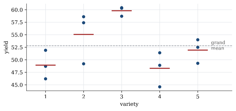
Example 1 (Five varieties of corn) Five varieties of corn are each grown on three plots.
| Variety | 1 | 2 | 3 | 4 | 5 |
|---|---|---|---|---|---|
| Yields | 46.2, 51.9, 48.7 | 49.2, 58.6, 57.4 | 60.3, 58.7, 60.4 | 48.9, 51.4, 44.6 | 52.5, 54.0, 49.3 |
| Mean | 48.93 | 55.07 | 59.80 | 48.30 | 51.93 |
Question. Do the varieties differ in mean yield?
Solution. The grand mean is 52.81. Then \mathrm{SS}_{\mathrm{treatment}}=3\sum_j(\overline y_{\cdot j}-52.81)^2=270.3 on 4 degrees of freedom, and \mathrm{SS}_{\mathrm{error}}=105.7 on 10.
| Source | Df | SS | MS | F | p |
|---|---|---|---|---|---|
| Variety | 4 | 270.3 | 67.57 | 6.39 | 0.008 |
| Error | 10 | 105.7 | 10.57 | ||
| Total | 14 | 375.9 |
The p-value is 0.008, so the varieties differ. The pooled standard deviation is \sqrt{10.57}=3.25. The F test says only that the five means are not all equal; which varieties differ is the next question.
Contrasts
Definition 2 (Contrast) A contrast is a linear combination C=\sum_j c_j\mu_j of the treatment means whose coefficients sum to zero. It is estimated by \widehat C=\sum_j c_j\overline Y_{\cdot j}, which is unbiased with variance \sigma^2\sum_j c_j^2/n_j.
A contrast tests a sub-hypothesis that was formulated before the data were seen. With \mathrm{SS}_C=\widehat C^2/\sum_jc_j^2/n_j, under H_0:C=0 the ratio \mathrm{SS}_C/\sigma^2 is \chi^2_1, independent of \mathrm{SS}_{\mathrm{error}}, so
F=\frac{\mathrm{SS}_C}{\mathrm{MS}_{\mathrm{error}}}
has the F_{1,\,n-k} distribution. The first part holds because \widehat C is normal with mean 0 under H_0, and \mathrm{SS}_C/\sigma^2 is its square over its variance. Contrasts that were chosen because the data suggested them do not keep that null distribution. A contrast has to be chosen from the scientific question, not from the ranking of the observed means.
Suppose varieties 1, 2, 4 and 5 of corn are mutations of one parent strain and variety 3 is not, so the question is whether variety 3 differs from the average of the others. The contrast is C=(\mu_1+\mu_2+\mu_4+\mu_5)/4-\mu_3, with estimate
\widehat C=\frac{48.93+55.07+48.30+51.93}{4}-59.80=-8.74,
and \sum c_j^2/n_j=(4/16+1)/3=0.4167. So F=(-8.74)^2/0.4167/10.57=17.4 on (1,10) degrees of freedom, with p-value 0.002. Variety 3 yields more than the mutant average.
Multiple comparisons
Comparing every pair of means with its own 95% interval inflates the chance that some interval misses. With five varieties there are ten pairs, and the chance that at least one of ten 95% intervals misses can be far above 5%. Tukey’s intervals control that simultaneous error.
Definition 3 (Tukey intervals) In a one-way design with k groups of equal size r, and n=kr, the probability is 1-\alpha that every one of the \binom k2 differences \mu_i-\mu_j simultaneously satisfies
\overline Y_{\cdot i}-\overline Y_{\cdot j}-D\sqrt{\mathrm{MS}_{\mathrm{error}}}<\mu_i-\mu_j<\overline Y_{\cdot i}-\overline Y_{\cdot j}+D\sqrt{\mathrm{MS}_{\mathrm{error}}}, \qquad D=\frac{Q_{k,\,n-k;\,1-\alpha}}{\sqrt r},
where Q_{k,\,n-k;\,1-\alpha} is the quantile of the studentised range for k groups and n-k error degrees of freedom.
The studentised range is the law of the largest minus the smallest of k independent standard normals, divided by an independent \sqrt{V/m} with V\sim\chi^2_m. Bounding the largest difference among the group means bounds all of them at once. A pair whose interval excludes zero is declared different at familywise level \alpha.
For the corn, k=5, r=3 and n-k=10, so Q_{5,10;0.95}=4.654 and the half-width of every interval is 4.654\sqrt{10.57/3}=8.74. The ten intervals for \mu_i-\mu_j are
| j=2 | j=3 | j=4 | j=5 | |
|---|---|---|---|---|
| i=1 | (-14.87,\ 2.60) | (-19.60,\ -2.13) | (-8.10,\ 9.37) | (-11.74,\ 5.74) |
| i=2 | (-13.47,\ 4.00) | (-1.97,\ 15.50) | (-5.60,\ 11.87) | |
| i=3 | (2.76,\ 20.24) | (-0.87,\ 16.60) | ||
| i=4 | (-12.37,\ 5.10) |
Two exclude zero: variety 3 yields more than variety 1 and more than variety 4. No other pair can be separated at familywise level 0.05.
Blocks
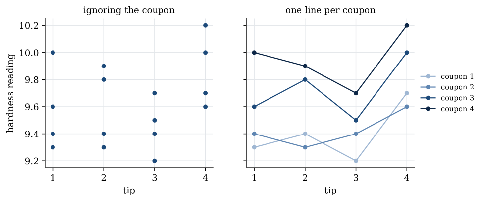
The hardness of a metal is measured by pressing a tester’s tip into a coupon of the metal. Four tips are each tested once on each of four coupons.
| Tip 1 | Tip 2 | Tip 3 | Tip 4 | |
|---|---|---|---|---|
| Coupon 1 | 9.3 | 9.4 | 9.2 | 9.7 |
| Coupon 2 | 9.4 | 9.3 | 9.4 | 9.6 |
| Coupon 3 | 9.6 | 9.8 | 9.5 | 10.0 |
| Coupon 4 | 10.0 | 9.9 | 9.7 | 10.2 |
Is there any difference between the tips? A one-way analysis with tip as the factor gives \mathrm{SS}_{\mathrm{tip}}=0.385 on 3 degrees of freedom and \mathrm{SS}_{\mathrm{error}}=0.905 on 12, so F=1.70 and p=0.22. No evidence of a difference.
But look at the coupons. Coupon 4 reads higher than coupon 1 under every tip. Much of the within-tip scatter is variation between coupons, and the one-way analysis lumps it into the error. Within each coupon, tip 4 reads highest and tip 3 lowest, almost every time.
Definition 4 (Randomised block design) A randomised block design measures every one of t treatments once in each of b blocks. The response for block i and treatment j is
Y_{ij}=\mu+\beta_i+\tau_j+\varepsilon_{ij}, \qquad \sum_{i=1}^b\beta_i=0,\quad\sum_{j=1}^t\tau_j=0,
with \varepsilon_{ij} independent and \operatorname{N}(0,\sigma^2). Here \mu is the overall mean, \beta_i the effect of block i and \tau_j the effect of treatment j.
The design is balanced: every block–treatment cell has the same number of observations, here one. The sums of squares are
\mathrm{SS}_{\mathrm{blocks}}=t\sum_{i=1}^b(\overline Y_{i\cdot}-\overline Y_{\cdot\cdot})^2, \qquad \mathrm{SS}_{\mathrm{treatment}}=b\sum_{j=1}^t(\overline Y_{\cdot j}-\overline Y_{\cdot\cdot})^2,
\mathrm{SS}_{\mathrm{error}}=\sum_{i=1}^b\sum_{j=1}^t(Y_{ij}-\overline Y_{i\cdot}-\overline Y_{\cdot j}+\overline Y_{\cdot\cdot})^2,
and the total splits as \mathrm{SS}_{\mathrm{total}}=\mathrm{SS}_{\mathrm{treatment}}+\mathrm{SS}_{\mathrm{blocks}}+\mathrm{SS}_{\mathrm{error}}, by the same cross-term argument as before. \mathrm{SS}_{\mathrm{error}}/\sigma^2 is \chi^2_{(b-1)(t-1)}. When every \tau_j=0, \mathrm{SS}_{\mathrm{treatment}}/\sigma^2 is \chi^2_{t-1}, and when every \beta_i=0, \mathrm{SS}_{\mathrm{blocks}}/\sigma^2 is \chi^2_{b-1}. The three are independent. So the treatment hypothesis is tested with
F=\frac{\mathrm{MS}_{\mathrm{treatment}}}{\mathrm{MS}_{\mathrm{error}}}\sim F_{t-1,\,(b-1)(t-1)},
and the block hypothesis with \mathrm{MS}_{\mathrm{blocks}}/\mathrm{MS}_{\mathrm{error}}\sim F_{b-1,\,(b-1)(t-1)}, each rejecting for large values.
For the hardness data, with coupons as blocks and tips as treatments:
| Source | Df | SS | MS | F | p |
|---|---|---|---|---|---|
| Coupon | 3 | 0.825 | 0.2750 | 30.94 | 0.00005 |
| Tip | 3 | 0.385 | 0.1283 | 14.44 | 0.0009 |
| Error | 9 | 0.080 | 0.00889 | ||
| Total | 15 | 1.290 |
The tip sum of squares is the same 0.385 as in the one-way analysis. What changed is the error. Of the one-way error sum of squares 0.905, 0.825 was variation between coupons. Removing it leaves 0.080, the error mean square falls from 0.075 to 0.0089, and the tips now differ very significantly. The large coupon sum of squares shows that blocking was worth doing. Contrasts and Tukey intervals carry over, with \mathrm{MS}_{\mathrm{error}} on (b-1)(t-1) degrees of freedom and D=Q_{t,\,(b-1)(t-1);\,1-\alpha}/\sqrt b. The true mean for treatment j is \mu+\tau_j, estimated by \overline Y_{\cdot j}; the mean for block i is \mu+\beta_i, estimated by \overline Y_{i\cdot}.
Two treatments: the paired t test
Two tyre types, A and B, are fitted one each to five cars, and the tread left after 10 000 km is measured.
| Car | 1 | 2 | 3 | 4 | 5 |
|---|---|---|---|---|---|
| Type A | 10.6 | 9.8 | 12.3 | 9.7 | 8.8 |
| Type B | 10.2 | 9.4 | 11.8 | 9.1 | 8.3 |
| Difference | 0.4 | 0.4 | 0.5 | 0.6 | 0.5 |
Wear depends heavily on the car and the driver, so this is a randomised block design with 5 blocks and 2 treatments. Under that model the within-car difference D_i=Y_{i1}-Y_{i2}=\tau_1-\tau_2+\varepsilon_{i1}-\varepsilon_{i2} is \operatorname{N}(\tau_1-\tau_2,\ 2\sigma^2), independently across cars, and the car effect has cancelled. Testing \tau_1=\tau_2 is a one-sample t test on the differences. Their mean is 0.48 and standard deviation 0.0837, so
t=\frac{0.48}{0.0837/\sqrt5}=12.8
on 4 degrees of freedom, with two-sided p-value 0.0002. The tyres differ in wear. The block F test gives F=164.6=12.8^2, the same test.
The completely randomised design is the several-group version of the two-sample t test. The block design is the several-treatment version of the paired t test.
Compare the variance of the group means with the variance inside the groups. Under equal means the ratio is an F statistic. Blocking pulls a known source of variation out of the error before that comparison is made.
A Bonferroni comparison and a worked haemoglobin table are in Analysis of variance examples.
Questions on this topic
Open a question to attempt it. Its worked answer is folded away at the bottom of the page.
What links here
Pages (5)
- Statistical inference — via analysis of variance
- Using R — via analysis of variance
- Analysis of variance examples — via Analysis of variance, Tukey intervals, Tukey’s method, randomised block design
- Linear model examples — via analysis of variance
- Paired comparisons, and how far a fit is from the data — via ANOVA
Questions and answers (8)