Chi-squared examples
Part of Data analysis · 2 questions on this topic · What links here
Chi-squared examples
| Part | Data analysis |
| Chapter | 9 of 9 in this part |
| Previous | Linear model examples |
| Questions | 2 |
| Figures | 1 |
The Pearson statistic, its chi-squared approximation, the loss of a degree of freedom for each estimated parameter, and the test of independence in a contingency table are in Chi-squared tests, where the frizzled chickens, the village houses and the ESP survey are worked by hand. This page checks the chi-squared approximation by simulation and runs the same tests in R.
Seeing the approximation
Example 1 (A hundred balls in ten boxes) Throw n=100 balls at random into k=10 boxes, each equally likely. The counts are multinomial, and each expected count is 10.
Question. What is the distribution of the Pearson statistic, and does it match \chi^2_9?
Solution. One throw gave the counts 14, 6, 13, 12, 11, 12, 5, 11, 7, 9, for which
T=\sum_{i=1}^{10}\frac{(x_i-10)^2}{10}=\frac{16+16+9+4+1+4+25+1+9+1}{10}=8.6.
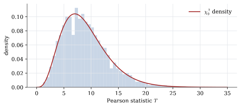
Repeating the experiment many times gives the distribution of T:
R <- 10000
t <- replicate(R, {
  counts <- tabulate(sample(1:10, size = 100, replace = TRUE), nbins = 10)
  sum((counts - 10)^2 / 10)
})
hist(t, breaks = 40, freq = FALSE)
curve(dchisq(x, df = 9), add = TRUE, col = 2, lwd = 2)
mean(t > qchisq(0.95, df = 9))     # close to 0.05
The histogram follows the \chi^2_9 density closely, and about 5% of the simulated statistics exceed the \chi^2_9 quantile 16.92, as they should under the null hypothesis. With 10 balls instead of 100, each expected count would be 1, far below the rule of thumb of 5, and the approximation would visibly fail.
Goodness of fit in R
chisq.test takes the observed counts and the hypothesised probabilities:
chisq.test(c(23, 50, 20), p = c(1/4, 1/2, 1/4))
# X-squared = 0.72043, df = 2, p-value = 0.6975
These are the frizzled chickens: the counts agree with the 1:2:1 ratio. When parameters have been estimated from the data, as for the Poisson fit to the village houses, chisq.test does not know it and reports k-1 degrees of freedom. Compute the statistic with it, then take the p-value from k-1-r degrees of freedom yourself, with pchisq(T, df = k - 1 - r, lower.tail = FALSE).
Independence in R
Given a matrix of counts, chisq.test tests independence of the row and column classifications:
esp <- matrix(c(67, 41, 6, 129, 183, 32), nrow = 2, byrow = TRUE,
              dimnames = list(c("Artist", "Non-artist"), c("Strong", "Moderate", "None")))
chisq.test(esp)
# X-squared = 15.936, df = 2, p-value = 0.0003462
chisq.test(esp)$expected   # the fitted counts R_i C_j / n
For a 2\times2 table R applies Yates’ continuity correction by default, which subtracts 1/2 from each |O-E| before squaring and makes the test more conservative. For 40 of 70 against 50 of 100,
tab <- matrix(c(40, 30, 50, 50), nrow = 2, byrow = TRUE)
chisq.test(tab)$statistic                   # 0.581, p = 0.446, corrected
chisq.test(tab, correct = FALSE)$statistic  # 0.843, p = 0.358, the Pearson statistic
The uncorrected statistic is the square of the two-proportion z statistic. When an expected count is small, R warns that the approximation may be poor; for a 2\times2 table fisher.test gives an exact test instead.
The chi-squared approximation is good when every expected count is about 5 or more, which a simulation makes visible. chisq.test computes the statistic; remember to subtract a degree of freedom for each estimated parameter, and that a 2\times2 table gets a continuity correction unless it is turned off.
Questions on this topic
Open a question to attempt it. Its worked answer is folded away at the bottom of the page.
| Question | Answer |
|---|---|
| Possums in five areas | ✓ |
| Genotype and mating success | ✓ |
What links here
Pages (1)
- Chi-squared tests — via Chi-squared examples