Regression examples
Part of Data analysis · 3 questions on this topic · What links here
Regression examples
| Part | Data analysis |
| Chapter | 7 of 9 in this part |
| Previous | Analysis of variance examples |
| Next | Linear model examples |
| Questions | 3 |
| Definitions | Multiple linear regression · Adjusted R-squared |
| Figures | 1 |
The least-squares line, the normal linear model, the t tests for the coefficients, and the intervals for a mean response and a new response are derived in Linear regression. This page fits regressions in R, reads every line of the summary, checks the residuals, and moves on to regression with more than one explanatory variable.
One explanatory variable
A survey of 100 students recorded, among other things, each student’s height in centimetres, shoe size in centimetres and weight in kilograms. Does shoe size help predict height?
Example 1 (Height and shoe size) Question. Fit the regression of height on shoe size and interpret the output.
Solution.
survey <- read.csv("studentsurvey.csv")
model1 <- lm(height ~ shoe, data = survey)
summary(model1)
# Residuals:
#      Min       1Q   Median       3Q      Max
# -18.9073  -6.1465   0.1096   6.3626  22.6384
# Coefficients:
#             Estimate Std. Error t value Pr(>|t|)
# (Intercept) 145.7776     5.7629  25.296  < 2e-16 ***
# shoe          1.0048     0.2178   4.613  1.2e-05 ***
# Residual standard error: 9.299 on 98 degrees of freedom
# Multiple R-squared:  0.1784,  Adjusted R-squared:  0.17
# F-statistic: 21.28 on 1 and 98 DF,  p-value: 1.199e-05
The fitted line is height =145.78+1.005\times shoe size: each extra centimetre of shoe goes with about one more centimetre of height, on average. Reading the rest:
- Residuals. The five-number summary of e_i=y_i-\widehat y_i. A median near 0 and quartiles roughly symmetric about it are what a normal error model predicts.
- Coefficients. Each estimate comes with its standard error, the t statistic estimate divided by standard error, and the two-sided p-value for the hypothesis that the coefficient is zero. For the slope, t=1.0048/0.2178=4.61 on 98 degrees of freedom, so shoe size is clearly associated with height. The test for the intercept, that the mean height is zero at shoe size zero, is meaningless here and is ignored.
- Residual standard error. The estimate S=9.3 cm of the error standard deviation \sigma: a typical student is about 9 cm from the line.
- R^2. Shoe size accounts for 17.8% of the variation in height. The relationship is real but explains little; most of the variation is elsewhere.
- F statistic. The test that every slope is zero. With one explanatory variable it is the square of the slope’s t, 4.613^2=21.28, with the same p-value.
Example 2 (Predicting a student’s height) Question. For a student with shoe size 30 cm, give a 95% interval for the mean height of such students, and a 95% interval for the height of one such student.
Solution.
predict(model1, data.frame(shoe = 30), interval = "confidence")
#        fit      lwr      upr
#   175.9217 173.4261 178.4172
predict(model1, data.frame(shoe = 30), interval = "prediction")
#        fit      lwr      upr
#   175.9217 157.2999 194.5434
The point prediction is 145.78+1.0048\times30=175.9 cm in both cases. The mean height of students with this shoe size is pinned down to within about 2.5 cm. A single student’s height is not: the prediction interval is (157.3,\ 194.5), about 37 cm wide, because a new student varies about the line with standard deviation near 9.3 cm whatever the sample size. The two intervals are the interval for the mean response and the prediction interval.
Checking the assumptions
The model assumes that, at each x, the responses are independent and normal, with a mean on a line and the same variance. The residuals are the evidence:
- a plot of residuals against fitted values (or against x) should be a patternless band of constant width around zero; a curve means the relationship is not linear, and a funnel means the variance grows with the mean;
- a normal quantile plot of the residuals should be close to a straight line;
- a few points far from the rest, or with unusual x values, deserve a second look, because a single point can move a least-squares line a long way.
plot(model1, 1:2) # residuals against fitted values, and a normal Q-Q plotA failed check is information. A curved residual plot suggests a transformation or an extra term in x^2; a funnel suggests modelling \log y; see the melanoma example in Linear regression.
Several explanatory variables
Definition 1 (Multiple linear regression) The multiple linear regression model for a response Y and explanatory variables x_1,\ldots,x_p is
Y_i=\beta_0+\beta_1x_{i1}+\cdots+\beta_px_{ip}+\varepsilon_i,\qquad\varepsilon_i\ \text{independent}\ \operatorname{N}(0,\sigma^2),
with the \beta_j estimated by least squares. The coefficient \beta_j is the change in mean response for a unit increase in x_j with the other explanatory variables held fixed.
“With the others held fixed” is the key phrase. A coefficient in a multiple regression answers a different question from the slope in a simple regression on the same variable, and the two can differ a great deal. The model is a special case of the linear model, and its matrix form is in Bayesian linear regression.
Definition 2 (Adjusted R-squared) For a regression with p explanatory variables on n observations, the adjusted R^2 is
R^2_{\mathrm{adj}}=1-(1-R^2)\frac{n-1}{n-p-1}.
Adding any variable can only raise R^2, even a column of random noise, because least squares can always use it to fit the sample a little better. The adjusted version charges for each parameter, and it falls when a new variable improves the fit by less than chance would.
Example 3 (Height, shoe size and weight) Question. Add weight to the regression of height on shoe size, and interpret both coefficients.
Solution.
model2 <- lm(height ~ shoe + weight, data = survey)
summary(model2)
#             Estimate Std. Error t value Pr(>|t|)
# (Intercept) 132.2677     5.2473  25.207  < 2e-16 ***
# shoe          0.5304     0.1962   2.703   0.0081 **
# weight        0.3744     0.0572   6.546 2.82e-09 ***
# Residual standard error: 7.785 on 97 degrees of freedom
# Multiple R-squared:  0.4301,  Adjusted R-squared:  0.4184
# F-statistic: 36.61 on 2 and 97 DF,  p-value: 1.429e-12
confint(model2)
#                   2.5 %      97.5 %
# (Intercept) 121.8533072 142.6821199
# shoe          0.1410087   0.9198251
# weight        0.2608887   0.4879514
Among students of the same weight, one more centimetre of shoe goes with 0.53 cm more height on average (p=0.008); among students with the same shoe size, one more kilogram goes with 0.37 cm more height (p=3\times10^{-9}). The shoe-size coefficient has roughly halved from the simple regression, because shoe size and weight are themselves related: part of what shoe size “explained” alone is now credited to weight. Together the two variables account for 43% of the variation in height, up from 18%, and the residual standard error falls from 9.3 to 7.8 cm. The adjusted R^2, 0.418, is barely below R^2, so the gain is not an artefact of adding a parameter.
For a student with shoe size 30 cm and weight 75 kg, predict(model2, data.frame(shoe = 30, weight = 75), interval = "conf") gives a mean height of 132.27+0.5304\times30+0.3744\times75=176.3 cm, with 95% interval (174.2,\ 178.4).
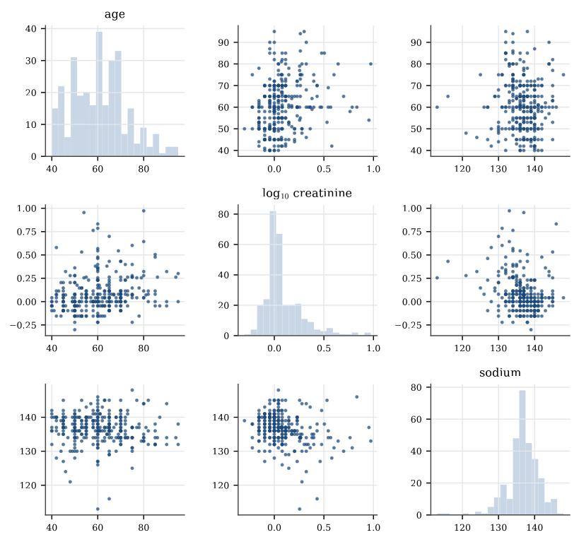
The scatterplot matrix, pairs(~ height + shoe + weight, data = survey), is the first look before a multiple regression: it shows which variables are related to the response, and which explanatory variables are related to each other, which is when coefficients change as variables are added.
Read a regression summary line by line: the estimate and its standard error, the t test that the coefficient is zero, the residual standard error, and R^2. Check the residuals before trusting any of it. In a multiple regression each coefficient is an effect with the other variables held fixed.
Questions on this topic
Open a question to attempt it. Its worked answer is folded away at the bottom of the page.
| Question | Answer |
|---|---|
| Height and age of pine trees | ✓ |
| Birth weight and mother’s age | ✓ |
| Rain, food, and orange yield | ✓ |
What links here
Pages (3)
- Linear regression — via Regression examples
- Linear model examples — via multiple regression
- Bayesian linear regression — via Regression examples
See also
- Articles from this chapter: Multiple linear regression · Adjusted R-squared
- All data analysis chapters
- Glossary and index
- Distribution sheet and formula lookup