Dependence along a series
Part of Time series · 7 questions on this topic · What links here
Dependence along a series
| Part | Time series |
| Chapter | 1 of 2 in this part |
| Next | Forecasting |
| Questions | 7 |
| Results | Wold decomposition |
| Figures | 1 |
Clustered data are dependent because they share a block. A time series is dependent because it is ordered. Today’s observation can depend on yesterday’s observation, or on yesterday’s surprise. The aim is less “describe this sample” than “say what happens next”. A perfect fit to the past, with one parameter per time point, does not forecast.
Autoregression and moving averages
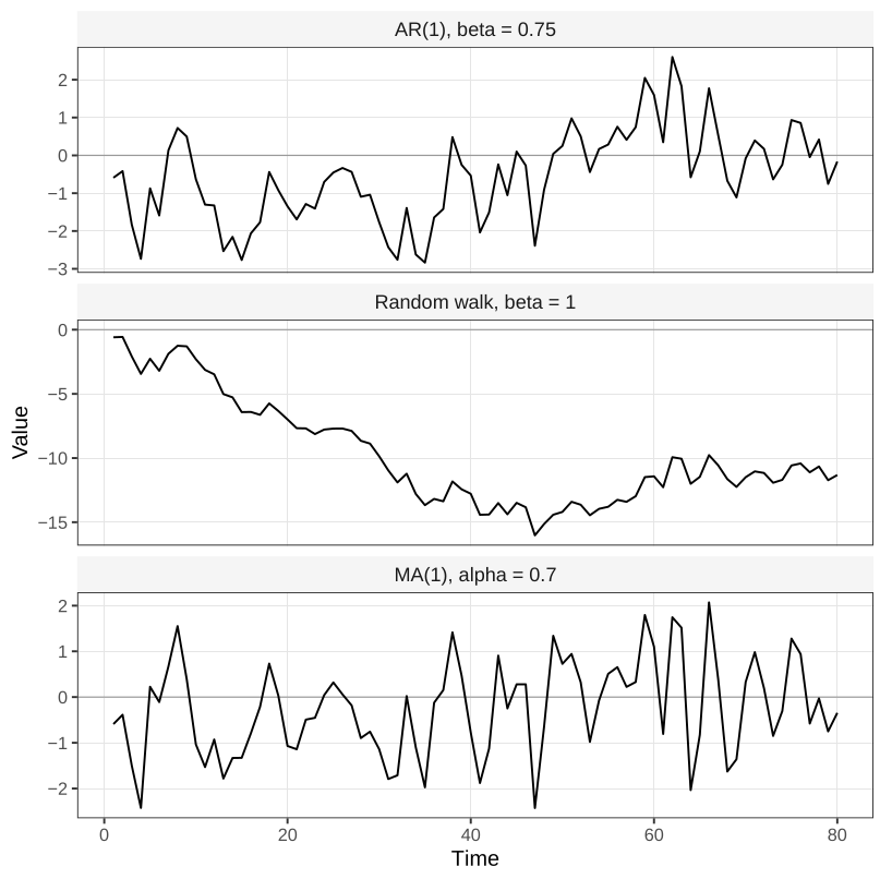
An autoregression of order 1 writes X_t=\beta X_{t-1}+\varepsilon_t, with the innovations \varepsilon_t independent of each other. A random walk is the case \beta=1, and it wanders off. A spring temperature might have \beta a little above 1, a drift toward summer, plus a daily innovation. A winter temperature might have \beta a little below 1. The best guess of today’s temperature, before the day is observed, is often yesterday’s. A Markov chain is the same skeleton: the next state depends on the current state and a draw.
A moving average of order 1 depends on the previous innovation rather than the previous level: X_t=\alpha\varepsilon_{t-1}+\varepsilon_t. Stock that did not sell yesterday, discounted and sold today, plus a new surplus, is that equation. So is a weather forecast whose credibility today depends on how wrong it was yesterday, with \alpha the weight on yesterday’s error.
A series we record is a finite piece of a process that could have been running for a long time, and often in continuous time. A city’s midday temperature on 365 days is a sample from a continuous temperature path, taken at one hour of each day. The whole process can be studied first, and finite collections of times examined afterwards, which is the probabilist’s direction. Or a model can be written for the finite collection observed, which is the statistical direction. If every finite subcollection is multivariate normal, the continuous-time process is a Gaussian process, and the converse holds too. That equivalence is special to the normal. It is also why a Gaussian-process prior has become a fashionable smoother: one draw of the process is a curve, and a penalty on how irregular the draw is plays the role of \lambda in the smoothing chapters.
Stationarity
Without some repetition, a series of length T does not identify a different mean at every time and a different covariance for every pair. Strict stationarity says that any block of observations has the same joint distribution as the same block shifted by \tau. The path changes. The distribution does not. Weak stationarity asks only for two moments: a mean \mu that does not depend on time, and a covariance that depends on the two times only through their difference, \gamma_{t-s}=\mathrm{Cov}(X_s,X_t). The lag-zero value \gamma_0=\mathrm{Var}(X_t) is then constant as well. The autocorrelation is \gamma_h/\gamma_0, which lies in [-1,1]. For a Gaussian process, weak stationarity and strict stationarity are the same statement. Otherwise weak is weaker.
The variogram looks at the change rather than the level: \mathrm{Var}(X_s-X_t)=2(\gamma_0-\gamma_{t-s}) when the process is weakly stationary. People often care about how much tomorrow moves from today, not about the variance of today’s temperature in isolation. A variogram can exist when the covariance function does not, because the difference X_s-X_t can be well behaved when X_t itself is not.
Theorem 1 If \{X_t\} is weakly stationary with mean zero, then X_t=\sum_{j=0}^{\infty} a_j\varepsilon_{t-j}+\nu_t, where the \varepsilon_t are uncorrelated with mean zero and variance \sigma^2, the coefficients a_j are constants, \nu_t is linearly determined by its own past, and the innovations are uncorrelated with \nu_t. If the mean is \mu, add \mu to the right-hand side.
Every weakly stationary series is a moving average of infinite order, plus a deterministic piece. In practice the mean is subtracted first and put back at the end. The modelling choices are then which of those pieces we keep: is the dependence Markov, or seasonal, or both; is the season only in the mean; are the lags added or multiplied? A multiplicative series is often logged, and then the forecast is on the log scale. Jensen’s inequality says \mathrm{E}(\log X)\neq\log\mathrm{E}(X). Exponentiating a forecast of the log is not a forecast of the mean on the original scale.
White noise is the building block inside that sum: uncorrelated innovations with mean zero and constant variance. The next chapter is a forecasting application rather than a further derivation of white noise, AR(p), and MA(q).
An AR(1) with coefficient 1 is a random walk. Say what happens to the variance of X_t as t grows, and why that process cannot be weakly stationary.
For a weakly stationary series, show \mathrm{Var}(X_s-X_t)=2(\gamma_0-\gamma_{|t-s|}) from the definition of \gamma.
Why does a time series of length T, with a different mean at each time and a free covariance for every pair, run out of degrees of freedom? What does weak stationarity put in place of those free parameters?
Questions on this topic
Open a question to attempt it. Its worked answer is folded away at the bottom of the page.
What links here
Pages (2)
- Markov chains, Gibbs sampling, and Metropolis–Hastings — via autocorrelation function
- Forecasting — via Wold decomposition, white noise, partial autocorrelation
Questions and answers (9)
See also
- Articles from this chapter: Wold decomposition
- All time series chapters
- Glossary and index
- Distribution sheet and formula lookup