Random variables and distributions
Part of Probability · 27 questions on this topic · What links here
Random variables and distributions
| Part | Probability |
| Chapter | 2 of 7 in this part |
| Previous | Random experiments and probability |
| Next | Simulation |
| Questions | 27 |
| Definitions | Random variable · Cumulative distribution function · Discrete distribution · Continuous distribution · Expectation · Variance · Probability generating function · Moment generating function · Bernoulli distribution · Binomial distribution · Geometric distribution · Poisson distribution · Hypergeometric distribution · Uniform distribution · Exponential distribution · Normal distribution · Gamma distribution |
| Results | Expectation of a function · Poisson limit of the binomial · Memoryless property |
| Figures | 3 |
A random variable is a numerical summary of an experiment. Once the sample space and the probability are fixed, the distribution of that summary is enough for any question that depends on the experiment only through the summary. Means, variances and the named families on the common distributions page are all statements about such summaries. This chapter says which experiment produces which family. The sheet records the probability function, the mean and the variance in the parameterisation used here. The second gamma parameter on that sheet is a rate. The geometric law there starts at 1.
Two families are not on the sheet, so their formulas are written out below: the uniform distribution on an interval, and the hypergeometric distribution.
Random variables
Definition 1 (Random variable) A random variable is a function X from the sample space \Omega to the real numbers. The event \{X\le x\} is the set of outcomes \omega with X(\omega)\le x.
Two dice have sample space \{1,\ldots,6\}^2. Their sum X(i,j)=i+j is a random variable with values in \{2,\ldots,12\}. The number of heads in n coin tosses is a random variable on \{0,1\}^n. The modelling gain is that later calculations can ignore the underlying outcomes and work with X alone.
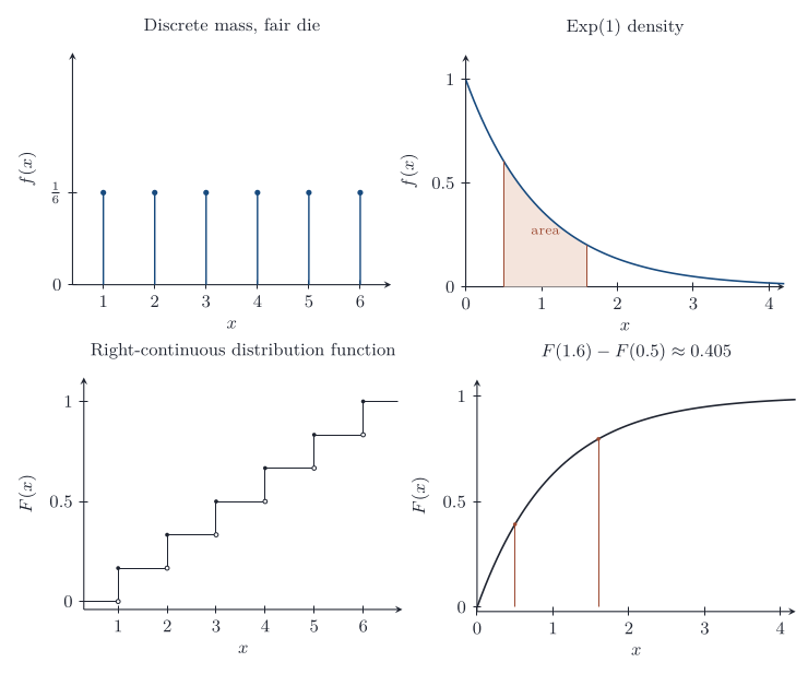
Definition 2 (Cumulative distribution function) The cumulative distribution function of X is F(x)=\mathbb{P}(X\le x), for x\in\mathbb{R}.
Every distribution function is non-decreasing, tends to 0 as x\to-\infty and to 1 as x\to\infty, and is right-continuous. Conversely, any function with those properties is the distribution function of some random variable. For a<b,
\mathbb{P}(a<X\le b)=F(b)-F(a).
Definition 3 (Discrete distribution) X is discrete when it takes values in a countable set S. Its probability mass function is f(x)=\mathbb{P}(X=x) for x\in S, and \mathbb{P}(X\in B)=\sum_{x\in B}f(x).
A fair die has mass function f(x)=1/6 on \{1,\ldots,6\}. The mass function determines the distribution function by adding the atoms up to x, and the jumps of the distribution function are the atoms.
Definition 4 (Continuous distribution) X is continuous when its distribution function can be written F(x)=\int_{-\infty}^{x} f(u)\,\,\mathrm{d} u for a non-negative function f with \int_{-\infty}^{\infty} f=1. The function f is a probability density. Then \mathbb{P}(X\in B)=\int_B f, and f=F' at every point where F is differentiable.
A density is not a probability. The probability of an infinitesimal interval (x,x+\,\mathrm{d} x) is about f(x)\,\,\mathrm{d} x. A single point still has probability zero. Drawing uniformly from [0,1] has density f(x)=1 on that interval and distribution function F(x)=x there.
Expectation and variance
Definition 5 (Expectation) If X is discrete with mass function f, its expectation is \mathbb{E} X=\sum_x x\,f(x), when the sum converges absolutely. If X is continuous with density f, \mathbb{E} X=\int_{-\infty}^{\infty} x\,f(x)\,\,\mathrm{d} x, when the integral converges absolutely.
The expectation is a centre of mass: point masses f(x) placed at the positions x balance at \mathbb{E} X. A symmetric mass function therefore has expectation at the centre of symmetry, when the expectation exists. The expectation need not be a value that X can take. A fair die has expectation 7/2.
Theorem 1 (Expectation of a function) If g is a real function and X is discrete with mass function f, then \mathbb{E} g(X)=\sum_x g(x)\,f(x). If X is continuous with density f, then \mathbb{E} g(X)=\int_{-\infty}^{\infty} g(x)\,f(x)\,\,\mathrm{d} x, whenever the sum or integral converges absolutely.
In the discrete case, group the outcomes on which g takes the value y. The mass at y is \sum_{x:g(x)=y}f(x), so \mathbb{E} g(X)=\sum_y y\sum_{x:g(x)=y}f(x)=\sum_x g(x)\,f(x).
Linearity is the useful consequence. For constants a and b, and functions g and h whose expectations exist,
\mathbb{E}(aX+b)=a\,\mathbb{E} X+b, \qquad \mathbb{E}\bigl(g(X)+h(X)\bigr)=\mathbb{E} g(X)+\mathbb{E} h(X).
No independence is required. Linearity is why a sum of indicators has expectation equal to the sum of the probabilities, even when the indicators are dependent.
Definition 6 (Variance) The variance of X is \operatorname{Var}(X)=\mathbb{E}(X-\mathbb{E} X)^2, when that expectation exists. Equivalently, \operatorname{Var}(X)=\mathbb{E} X^2-(\mathbb{E} X)^2. The standard deviation is the square root of the variance.
Variance measures spread about the expectation. It scales by the square of a constant: \operatorname{Var}(aX+b)=a^2\operatorname{Var}(X). The shift b does not appear, because variance ignores location.
Transforms
Definition 7 (Probability generating function) If N takes values in \{0,1,2,\ldots\}, its probability generating function is G(z)=\mathbb{E} z^N=\sum_{n=0}^{\infty}\mathbb{P}(N=n)\,z^n, for |z|\le 1.
The mass function can be recovered by differentiation at the origin: \mathbb{P}(N=n)=G^{(n)}(0)/n!. The mean and variance sit at the other endpoint, when they exist:
\mathbb{E} N=G'(1), \qquad \operatorname{Var}(N)=G''(1)+G'(1)-\bigl(G'(1)\bigr)^2.
For a fair comparison with the sheet, the generating functions of the named non-negative integer laws are (1-p+zp) for a Bernoulli trial, (1-p+zp)^n for a binomial count, zp/(1-(1-p)z) for a geometric count that starts at 1, and e^{\lambda(z-1)} for a Poisson count.
Definition 8 (Moment generating function) The moment generating function of X is M(s)=\mathbb{E} e^{sX}, for those s at which the expectation exists.
If M exists in an open interval around 0, it determines the distribution, and the moments are derivatives at the origin: \mathbb{E} X^n=M^{(n)}(0). The practical use is addition. If X and Y are independent, then M_{X+Y}(s)=M_X(s)M_Y(s) wherever both factors exist. That is often the shortest proof that a sum stays inside a family.
Named distributions
A handful of distributions recur because a handful of experiments recur. Each is listed with the experiment it describes, and its mean and variance are derived from the generating functions above, so the formulas on the common distributions page can be rebuilt rather than memorised.
Bernoulli and binomial
Definition 9 (Bernoulli distribution) X has the Bernoulli distribution with success probability p\in[0,1], written X\sim\operatorname{Bern}(p), when \mathbb{P}(X=1)=p and \mathbb{P}(X=0)=1-p. Then \mathbb{E} X=p and \operatorname{Var}(X)=p(1-p).
A Bernoulli variable records a single trial: success as 1, failure as 0. Because X^2=X, \mathbb{E} X^2=p and \operatorname{Var}(X)=p-p^2. The variance is largest, 1/4, at p=1/2, where the outcome is least predictable.
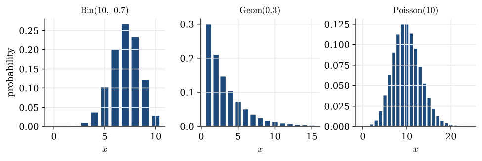
Definition 10 (Binomial distribution) X has the binomial distribution with n trials and success probability p, written X\sim\operatorname{Bin}(n,p), when
\mathbb{P}(X=x)=\binom nx p^x(1-p)^{n-x},\qquad x=0,1,\ldots,n.
It is the number of successes in n independent \operatorname{Bern}(p) trials. Then \mathbb{E} X=np and \operatorname{Var}(X)=np(1-p).
The mass function is the coin-toss count of Random experiments and probability: each sequence with x successes has probability p^x(1-p)^{n-x}, and there are \binom nx of them. The moments are quickest from the generating function. Writing X=X_1+\cdots+X_n for the n independent trials, each with generating function 1-p+pz,
G(z)=(1-p+pz)^n,\qquad G'(1)=np,\qquad G''(1)=n(n-1)p^2,
so \mathbb{E} X=np and \operatorname{Var}(X)=n(n-1)p^2+np-n^2p^2=np(1-p). The same answer follows without generating functions: the mean of a sum is the sum of the means, and the variance of a sum of independent terms is the sum of the variances.
Example 1 (Defective items in a box) Each item from a production line is defective with probability 0.05, independently of the others. A box holds 20 items.
Question. Find the expected number of defective items in a box, and the probability that a box has at most one.
Solution. The number of defectives is X\sim\operatorname{Bin}(20,0.05), so \mathbb{E} X=20\times0.05=1. Then
\mathbb{P}(X\le1)=0.95^{20}+20\times0.05\times0.95^{19}=0.358+0.377=0.736.
Although the average is exactly one defective, more than a quarter of boxes have two or more.
Geometric
Definition 11 (Geometric distribution) X has the geometric distribution with success probability p\in(0,1], written X\sim\operatorname{Geom}(p), when
\mathbb{P}(X=x)=(1-p)^{x-1}p,\qquad x=1,2,\ldots
It is the trial on which the first success occurs, in a sequence of independent \operatorname{Bern}(p) trials. Then \mathbb{E} X=1/p and \operatorname{Var}(X)=(1-p)/p^2.
The first success is at trial x exactly when the first x-1 trials fail and trial x succeeds, which gives the mass function, and \mathbb{P}(X>x)=(1-p)^x because that happens when the first x trials fail. With q=1-p the generating function is a geometric series,
G(z)=\sum_{x=1}^\infty q^{x-1}p\,z^x=\frac{pz}{1-qz},\qquad G'(z)=\frac{p}{(1-qz)^2},\qquad G''(z)=\frac{2pq}{(1-qz)^3}.
So \mathbb{E} X=G'(1)=1/p and \operatorname{Var}(X)=2q/p^2+1/p-1/p^2=q/p^2. A fair die needs six throws on average to show its first six. Some books count the failures before the first success instead, X-1, which has mean (1-p)/p; the two conventions differ by exactly one.
Poisson
Definition 12 (Poisson distribution) X has the Poisson distribution with mean \lambda>0, written X\sim\operatorname{Poisson}(\lambda), when
\mathbb{P}(X=x)=e^{-\lambda}\frac{\lambda^x}{x!},\qquad x=0,1,2,\ldots
Then \mathbb{E} X=\operatorname{Var}(X)=\lambda.
Theorem 2 (Poisson limit of the binomial) If X_n\sim\operatorname{Bin}(n,p_n) with np_n\to\lambda as n\to\infty, then \mathbb{P}(X_n=x)\to e^{-\lambda}\lambda^x/x! for every x=0,1,2,\ldots
Write p_n=\lambda_n/n with \lambda_n\to\lambda. Then
\binom nx p_n^x(1-p_n)^{n-x}=\frac{\lambda_n^x}{x!}\cdot\frac{n(n-1)\cdots(n-x+1)}{n^x}\cdot\Bigl(1-\frac{\lambda_n}n\Bigr)^n\Bigl(1-\frac{\lambda_n}n\Bigr)^{-x}.
As n\to\infty the second factor tends to 1, the third to e^{-\lambda} and the fourth to 1. That is why the Poisson law models the number of rare events in a fixed interval of time or space: many independent chances, each small, with a steady average number of successes. Calls to an exchange, decays of a radioactive sample and typing errors on a page are the standard examples.
The generating function is G(z)=\sum_x e^{-\lambda}(\lambda z)^x/x!=e^{\lambda(z-1)}. Then G'(1)=\lambda and G''(1)=\lambda^2, so the mean is \lambda and the variance is \lambda^2+\lambda-\lambda^2=\lambda. Equal mean and variance is the signature of a Poisson count, and data whose variance is well above the mean are called overdispersed; see Standard errors, and models for counts.
Example 2 (A rare fault) A machine makes 1000 parts a day, and each part has a fault with probability 0.002, independently.
Question. Find the probability that a day has at most one faulty part, exactly and by the Poisson approximation.
Solution. The exact count is \operatorname{Bin}(1000,0.002), and \mathbb{P}(X\le1)=0.998^{1000}+1000\times0.002\times0.998^{999}=0.4057. The Poisson approximation uses \lambda=1000\times0.002=2:
\mathbb{P}(X\le1)\approx e^{-2}(1+2)=0.4060.
The two agree to three decimal places. The approximation is good whenever n is large and p is small, and it needs only the product np.
Hypergeometric
Definition 13 (Hypergeometric distribution) A hypergeometric count draws n items without replacement from a population of size N that contains r marked items. If X is the number of marked items in the draw, then
\mathbb{P}(X=x)=\frac{\binom{r}{x}\binom{N-r}{n-x}}{\binom{N}{n}},
for every integer x with \max(0,n-(N-r))\le x\le\min(n,r). Write p=r/N. Then \mathbb{E} X=np and
\operatorname{Var}(X)=np(1-p)\frac{N-n}{N-1}.
The mass function counts the ways to choose x of the marked items and n-x of the others, over the ways to choose any n. The mean matches the with-replacement, binomial, experiment. The variance is smaller by the factor (N-n)/(N-1), which is the effect of not putting items back. When the population is much larger than the sample, the factor is close to 1 and the binomial is a good approximation.
Example 3 (Aces in a hand) Five cards are dealt from a well-shuffled deck of 52.
Question. Find the distribution of the number of aces, and compare it with the binomial count for five draws with replacement.
Solution. The number of aces is hypergeometric with N=52, r=4 and n=5. For example,
\mathbb{P}(X=1)=\frac{\binom41\binom{48}4}{\binom{52}5}=\frac{4\times194580}{2598960}=0.2995.
The full distribution is 0.6588, 0.2995, 0.0399, 0.0017 and 0.00002 for 0 to 4 aces. The binomial count \operatorname{Bin}(5,1/13) gives 0.6702, 0.2792 and 0.0465 for 0 to 2. Both have mean 5/13=0.385, but without replacement each ace drawn makes the next less likely, so the hypergeometric count is less spread out.
Uniform
Definition 14 (Uniform distribution) X is uniform on the interval [a,b], written X\sim\operatorname{U}[a,b], when its density is 1/(b-a) on that interval and zero elsewhere. Then \mathbb{E} X=(a+b)/2 and \operatorname{Var}(X)=(b-a)^2/12.
The continuous analogue of an equally likely finite set is the uniform distribution: probability is proportional to length. The distribution function rises linearly from 0 to 1 across [a,b]. For the moments, \mathbb{E} X^2=\int_a^bx^2\,\,\mathrm{d} x/(b-a)=(a^2+ab+b^2)/3, and subtracting ((a+b)/2)^2 leaves (b-a)^2/12. The uniform law on [0,1] is the raw material of simulation.
Exponential
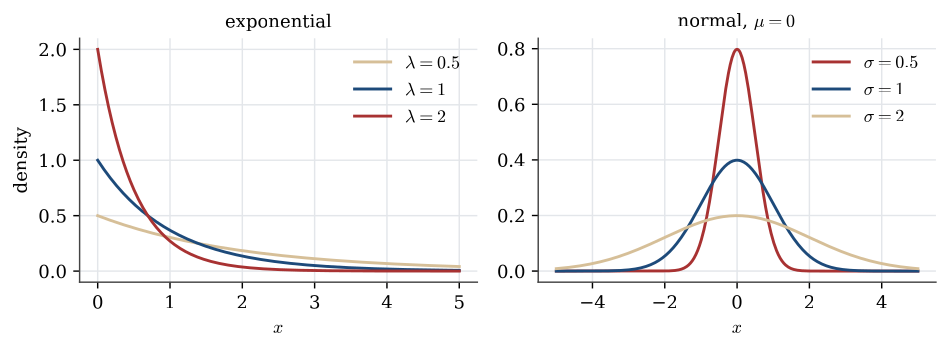
Definition 15 (Exponential distribution) X has the exponential distribution with rate \lambda>0, written X\sim\operatorname{Exp}(\lambda), when its density is \lambda e^{-\lambda x} for x>0. Its distribution function is 1-e^{-\lambda x}, its mean is 1/\lambda and its variance is 1/\lambda^2.
The moment generating function is M(s)=\int_0^\infty e^{sx}\lambda e^{-\lambda x}\,\mathrm{d} x=\lambda/(\lambda-s) for s<\lambda. Then M'(0)=1/\lambda and M''(0)=2/\lambda^2, so the variance is 2/\lambda^2-1/\lambda^2=1/\lambda^2. The exponential law is the usual model for a waiting time that does not age, and its defining property is the next theorem.
Theorem 3 (Memoryless property) A positive random variable X is memoryless when \mathbb{P}(X>s+t\mid X>s)=\mathbb{P}(X>t) for all s,t>0. The exponential distributions are the continuous memoryless laws, and the geometric distributions are the discrete ones.
For the exponential law with rate \lambda, the survival probability is e^{-\lambda x}, so
\mathbb{P}(X>s+t\mid X>s)=\frac{e^{-\lambda(s+t)}}{e^{-\lambda s}}=e^{-\lambda t}.
The geometric calculation is the same with (1-p)^{s+t} in place of e^{-\lambda(s+t)}.
Memorylessness is a modelling claim. A component whose lifetime is exponential does not become more likely to fail as it gets older. The failure rate is constant. A bulb with exponential lifetime of mean 1000 hours that has already burned for 1000 hours survives another 500 with probability e^{-500/1000}=0.607, the same as a new bulb. Lifetime models that do age are on the reliability page.
Normal
Definition 16 (Normal distribution) X has the normal distribution with mean \mu and variance \sigma^2>0, written X\sim\operatorname{N}(\mu,\sigma^2), when its density is
\frac1{\sigma\sqrt{2\pi}}\exp\Bigl\{-\frac{(x-\mu)^2}{2\sigma^2}\Bigr\},\qquad x\in\mathbb{R}.
The standard normal distribution is \operatorname{N}(0,1), with distribution function written \Phi.
The density is a bell centred at \mu, with inflection points at \mu\pm\sigma. An affine image of a normal variable is normal: if X\sim\operatorname{N}(\mu,\sigma^2) and a\ne 0, then aX+b\sim\operatorname{N}(a\mu+b,a^2\sigma^2). The moment generating function M(s)=\exp(\mu s+\sigma^2 s^2/2) makes this immediate, and it is proved again from the transformation rule in Functions of random variables and limit theorems.
The practical consequence is standardisation. If X\sim\operatorname{N}(\mu,\sigma^2) then Z=(X-\mu)/\sigma is standard normal, so every normal probability is a value of \Phi:
\mathbb{P}(a<X\le b)=\Phi\Bigl(\frac{b-\mu}\sigma\Bigr)-\Phi\Bigl(\frac{a-\mu}\sigma\Bigr).
By symmetry \Phi(-z)=1-\Phi(z), so tables list only z\ge0. A normal variable falls within one standard deviation of its mean with probability 0.683, within two with probability 0.954, and within three with probability 0.997.
Example 4 (IQ scores) Suppose IQ scores are \operatorname{N}(100,16^2).
Question. What fraction of people score between 90 and 110, and what fraction above 130?
Solution. Standardise: (90-100)/16=-0.625 and (110-100)/16=0.625, so
\mathbb{P}(90<X\le110)=\Phi(0.625)-\Phi(-0.625)=2\Phi(0.625)-1=0.468.
Above 130, z=1.875 and \mathbb{P}(X>130)=1-\Phi(1.875)=0.030, about one person in 33. These are the class probabilities used to sort recruits in Chi-squared tests.
Gamma and chi-squared
Definition 17 (Gamma distribution) X has the gamma distribution with shape \alpha>0 and rate \lambda>0, written X\sim\operatorname{Gamma}(\alpha,\lambda), when its density is
\frac{\lambda^\alpha x^{\alpha-1}e^{-\lambda x}}{\Gamma(\alpha)},\qquad x>0,
where \Gamma(\alpha)=\int_0^\infty u^{\alpha-1}e^{-u}\,\mathrm{d} u. Then \mathbb{E} X=\alpha/\lambda and \operatorname{Var}(X)=\alpha/\lambda^2.
Integration by parts gives \Gamma(\alpha+1)=\alpha\Gamma(\alpha), and \Gamma(1)=1, so \Gamma(k)=(k-1)! for whole numbers k; also \Gamma(1/2)=\sqrt\pi. The exponential law is the gamma law with shape 1. The moment generating function is M(s)=(\lambda/(\lambda-s))^\alpha for s<\lambda, so independent gamma variables with a common rate add their shapes. In particular, a sum of k independent \operatorname{Exp}(\lambda) waiting times is \operatorname{Gamma}(k,\lambda), the time of the kth event. A chi-squared variable with k degrees of freedom, used throughout Statistical inference, is the gamma law with shape k/2 and rate 1/2.
The time S_k of the kth event is longer than t exactly when fewer than k events have happened by time t. With events arriving at rate \lambda, that count is \operatorname{Poisson}(\lambda t), so
\mathbb{P}(S_k>t)=\sum_{j=0}^{k-1}e^{-\lambda t}\frac{(\lambda t)^j}{j!}.
For three events at rate 2 per hour, the probability that the third takes more than 2 hours is e^{-4}(1+4+8)=0.238.
The distribution is the probability of the events \{X\in B\}. Discrete distributions are specified by a mass function, continuous distributions by a density. The expectation of a function is the average of that function against the mass or the density, and linearity does not need independence.
Questions on this topic
Open a question to attempt it. Its worked answer is folded away at the bottom of the page.
What links here
Pages (23)
- Random experiments and probability — via binomial distribution, geometric distribution
- Simulation — via distribution function, Random variables and distributions, Bernoulli trial, binomial distribution
- Joint distributions — via random variables, probability mass function, expectation, moment generating function
- Functions of random variables and limit theorems — via random variable, distribution function, moment generating function, expectation
- Reliability — via Random variables and distributions, binomial distribution, distribution function, random variable
- Statistical inference — via Random variables and distributions, random variables, mass function, expectations
- Estimation — via Bernoulli trials, density function, mass function, uniform distribution
- Chi-squared tests — via expectations
- Linear regression — via random variable, expectations, normal distribution
- Analysis of variance — via expectation
- Studies, data, and evidence — via Random variables and distributions, expectations
- Descriptive statistics — via normal distribution
- Using R — via distribution functions
- The Beta–Binomial model — via Binomial distribution
- Conjugate analysis for normal models — via Gamma distribution
- Categorical data and the Dirichlet distribution — via Bernoulli trial, binomial distribution
- Bayesian linear regression — via normal distribution
- Introduction to generalised linear models — via gamma distribution, Bernoulli distribution, normal distribution
- Standard errors, and models for counts — via Poisson distribution, gamma distribution
- Paired comparisons, and how far a fit is from the data — via Poisson distribution
- Probability-integral residuals — via normal distribution
- Random slopes, and a binary mixed model — via normal distribution
- Marginal models, and two responses at once — via Poisson distribution
Questions and answers (53)
- The smaller face · The larger coordinate · A cubic distribution function · The sum of two dice · The waiting time itself · Particles in an hour (answer) · Three-point expectation · Recovering the second moment · Expected number of red balls (answer) · Expected wait for double six (answer) · Groups of three (answer) · A memoryless component · Exponential moments from the transform · A game on the sum of two dice · Two components with the same mean life (answer) · A game on the smaller face · Draws from an exponential law · Draws from a uniform interval · Rescaling a standard normal draw · A shifted exponential density · Minimum and average of uniform draws · A joint table · Distribution function of a maximum · The square of a binomial count · A normal law with mean 2 · State the probability functions · The sum of uniform draws · Ten successive exponential components · A walk with a floor (answer) · A string of twenty bulbs · Mean life as an integral of survival (answer) · An exponential rate · Counting degrees of freedom · Home-ground wins · Q2 · Q25 (answer) · Q28 (answer) · Q29 · Q45 (answer) · Q48 (answer) · Q49 · Q55 (answer) · Q56 (answer) · Question 1 (answer) · Question 4 · Question 5 (answer) · Question 8 · Question 9 (answer) · Question 17 · Question 20 (answer) · Question 21 (answer) · C22 (answer) · C23 (answer)
See also
- Articles from this chapter: Random variable · Cumulative distribution function · Discrete distribution · Continuous distribution · Expectation · Expectation of a function · Variance · Probability generating function · Moment generating function · Bernoulli distribution · Binomial distribution · Geometric distribution · Poisson distribution · Poisson limit of the binomial · Hypergeometric distribution · Uniform distribution · Exponential distribution · Memoryless property · Normal distribution · Gamma distribution
- All probability chapters
- Glossary and index
- Distribution sheet and formula lookup