Question 21. Cholesterol and heart disease
2025 examination, Question 3 (20 marks).
The heart-disease GAM is fitted by the following command, with the output shown below.
library(mgcv)
fit.sm1 = gam(disease ~ gender + s(cholesterol), family=binomial)

Parametric coefficients:
             Estimate Std. Error z value Pr(>|z|)
(Intercept)  -0.12716    0.32518  -0.391    0.696
gender       -0.08167    0.49478  -0.165    0.869

Approximate significance of smooth terms:
                edf Ref.df Chi.sq p-value
s(cholesterol) 2.011  2.537  18.21 0.00036 ***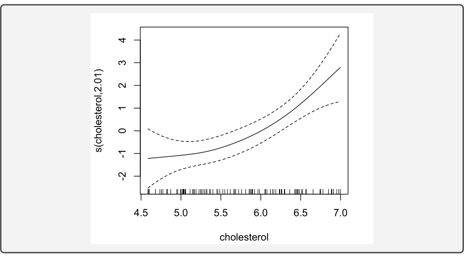
(a) [4 marks] Write the model statement for this command.
(b) [2 marks] Interpret the edf of 2.011.
(c) [2 marks] Test for a gender difference after accounting for cholesterol.
(d) [2 marks] Test whether a simple linear logistic regression on cholesterol is adequate.
(e) [3 marks] In light of (c) and (d), how would you simplify the model? Give the R command.
Another statistician instead fits
fit.sm2 = gam(disease ~ s(cholesterol), family=binomial(link="probit"))(f) [3 marks] Write the statistical model corresponding to this command.
The dashed curve below is the probit fit from (f); the solid curve is the simplified logit fit from (e).
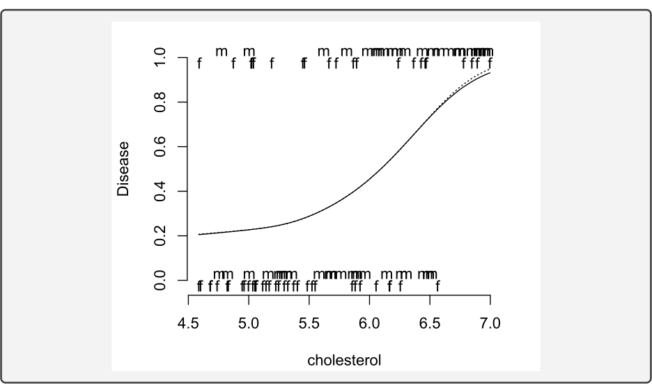
(g) [4 marks] Comment on the comparison and why the two fits look that way.
Definitions. Y_i is the disease indicator, c_i is cholesterol and G_i is the recorded gender covariate. The response probability is p_i=\mathbb{P}(Y_i=1\mid c_i,G_i). A GAM adds a fitted smooth to the linear predictor while retaining a response distribution and link function. Effective degrees of freedom describe the smooth’s flexibility after penalisation; they are not the polynomial degree.
(a) Naming binomial and not naming a link selects the logit. Let G_i denote the gender covariate as coded in the fitted dataset; the printed output does not identify its reference category.
\begin{aligned} Y_i\mid X_i &\sim \operatorname{Bernoulli}(p_i),\\ \operatorname{logit}(p_i) &= \beta_0+\beta_1 G_i+g(\mathrm{cholesterol}_i). \end{aligned}
The function g is a centred penalised smooth. Thus \beta_0 is the log-odds for the reference gender at zero contribution from the fitted smooth, not necessarily at a particular observed cholesterol value. Conditional on the covariates, responses are modelled as independent Bernoulli variables. The smooth replaces a single cholesterol slope.
For an ordinary smooth, a constraint such as \sum_i g(c_i)=0 separates it from the intercept. Without a constraint, adding a constant to g and subtracting that constant from \beta_0 would give the same fitted predictor. The plotted smooth is on the log-odds scale. To obtain a probability, form the entire predictor \eta_i=\beta_0+\beta_1G_i+g(c_i) and then calculate p_i=\operatorname{expit}(\eta_i); g(c_i) alone is neither a probability nor a probability difference.1
(b) The edf 2.011 measures the effective flexibility of the fitted cholesterol effect after penalisation. A value near 1 would be nearly linear on the logit scale; 2.011 suggests curvature. It does not mean that the fit is a quadratic polynomial. The reference df 2.537 belongs to the approximate test of the smooth term and is not another measure of its shape.
(c) The gender coefficient is -0.0817, with z=-0.165 and p=0.869. At a common cholesterol level, the fitted odds for the category coded 1 are \exp(-0.0817)\approx 0.92 times those for the reference category, assuming a 0/1 coding. The output does not show which category is coded 1. There is no evidence here of a gender difference after accounting for cholesterol.
The hypotheses are H_0:\beta_1=0 and H_1:\beta_1\ne0. The Wald statistic is the estimate divided by its standard error, and the two-sided normal-reference p-value is 2\{1-\Phi(|z|)\}. Since 0.869>0.05, do not reject the null at the 5\% level. This is insufficient evidence of an adjusted gender difference, rather than evidence that the difference is exactly zero.
(d) The printed \chi^2=18.21 and p=0.00036 test whether the cholesterol smooth is absent; they do not test whether it is linear.2 The two null hypotheses are different:
H_{0,\mathrm{absent}}:g(c)\equiv0,\qquad H_{0,\mathrm{linear}}:g(c)\text{ is a straight-line function of }c.
A nonzero straight line violates the first null but satisfies the second. Thus the small printed p-value establishes evidence of a cholesterol contribution under the model, while the curved plot and edf 2.011 suggest departures from linearity. A formal test of that narrower claim needs an appropriately calibrated comparison or decomposition of the nonlinear part. Keep the other covariates fixed in that comparison: the linear counterpart to the supplied model is glm(disease ~ gender + cholesterol, family=binomial). The required comparison statistic is not printed, so a formal p-value for nonlinearity cannot be supplied from this output alone.
(e) The gender term can be dropped for a simpler description of these data, while the plotted curvature supports retaining the cholesterol smooth. The simplified logit model is
gam(disease ~ s(cholesterol), family=binomial).
This is a parsimonious description supported by the supplied results, rather than proof of a unique correct model. It retains the Bernoulli assumptions and logit link. Removing the smooth instead would assert no cholesterol effect, contrary to its strong reported evidence.
(f) The probit link replaces the logistic curve by the standard normal distribution function \Phi:
\begin{aligned} Y_i\mid x_i &\sim \operatorname{Bernoulli}(p_i),\\ \Phi^{-1}(p_i) &= \widetilde\beta_0+\widetilde g(\mathrm{cholesterol}_i), \end{aligned}
with \widetilde g centred and with no gender term. Here \Phi is the standard normal CDF, so equivalently p_i=\Phi\{\widetilde\beta_0+\widetilde g(c_i)\}. The tildes emphasise that the intercept and smooth are fitted again under the new link; their numerical values need not match the logit fit. Changing the link leaves the Bernoulli response distribution unchanged.
(g) Both curves estimate disease probability as a smooth function of cholesterol alone. Logistic and normal CDFs are both sigmoid-shaped and symmetric about probability one half, although their numerical predictor scales and tail behaviour differ. Refitting the intercept and smooth can absorb much of that scale difference, explaining the very similar fitted probabilities over the observed cholesterol range. The curves need not agree when the same numerical predictor is inserted into each inverse link, or when extrapolated beyond the data.
The simplified logit and probit fits have the same covariates, so their displayed difference reflects the choice of link together with refitting under that link. A routine nested-model likelihood-ratio reference is not justified by treating one link as a parameter restriction of the other. AIC or an appropriate predictive comparison can be used if a formal model choice is required. The figure alone supplies little reason to prefer the probit fit.
The logit has a convenient interpretation: at two cholesterol values c_1,c_2, the fitted odds ratio is \exp\{g(c_2)-g(c_1)\}. With a smooth there is no single constant cholesterol odds ratio per unit increase; it depends on the two cholesterol values compared. This interpretability, together with the close fitted curves, supports reporting the logit model here.
Footnotes
The ordinary smooth constraint is described in the mgcv identifiability documentation.↩︎
The mgcv summary documentation defines smooth-term tests and explains the approximate nature of their p-values.↩︎