Three species on one hillside
Part of Correlated data · What links here
Three species on one hillside
loglinb3.| Part | Correlated data |
| Chapter | 4 of 4 in this part |
| Previous | Marginal models, and two responses at once |
| Figures | 1 |
The burn example had two different kinds of measurement on one child. This chapter stays with a vector response, but now every component is binary.
Thomas Yee’s VGAM package fits vector generalised linear models in which every component has the same type. It will not take one binary margin and one continuous margin, which is why the burn data were fitted by hand. It will take three binary margins. The Hunua ranges data record, at 392 locations, whether each of three New Zealand plants was present: Cyathea dealbata (cyadea), Beilschmiedia tawa (beitaw), and Knightia excelsa (kniexc). Altitude is the covariate. The plants may prefer different heights, and they may help or crowd each other, so the three binary responses at one location are not independent. The association is not forced to be positive.
Each margin is a logistic regression with its own intercept and its own slope on altitude: \mathrm{P}(Y_k=1\mid \text{altitude}) =\frac{\exp(\beta_{k0}+\beta_{k1}\,\text{altitude})}{1+\exp(\beta_{k0}+\beta_{k1}\,\text{altitude})}, and the working variance is the Bernoulli variance \mu_k(1-\mu_k). The working association between each pair is a log odds ratio: the odds of finding species k when species k' is present, divided by the odds of finding species k when species k' is absent. That is a two-way interaction. A three-way odds ratio, all three plants at once, can be written down but has no clear interpretation, so the working model stops at pairs. Any three species on a hillside do interact as a triple. The working model is therefore wrong. It does not have to be right for the slopes, once the sandwich standard errors are used.
vglm with the trivariate binary family loglinb3 returns model-based standard errors that assume the working variance and the working odds ratios. The sandwich is a plug-in on top of that fit. Altitude in the table is scaled by 10^3. In the coefficient vector, predictor 1 is Cyathea, 2 is Beilschmiedia, and 3 is Knightia. Predictors 4 to 6 are the pairwise log odds ratios. The slope table below keeps the three species intercepts and the three altitude slopes. The Std. Error column from summary is the naive standard error. The sandwich column in that table is the robust standard error.
need <- function(pkg) {
  if (!requireNamespace(pkg, quietly = TRUE)) {
    install.packages(pkg, repos = "https://cloud.r-project.org")
  }
  suppressPackageStartupMessages(library(pkg, character.only = TRUE))
}
need("VGAM")
data(hunua, package = "VGAM")
hunua$altkm <- hunua$altitude / 1000
summary(vglm(cbind(cyadea, beitaw, kniexc) ~ altkm,
family = loglinb3, data = hunua))| species | term | estimate | naive SE | sandwich SE | sandwich z |
|---|---|---|---|---|---|
| Cyadea | intercept | -0.977 | 0.222 | 0.170 | -5.74 |
| Cyadea | altitude \times 10^3 | -0.570 | 0.921 | 0.813 | -0.70 |
| Beitaw | intercept | -1.890 | 0.265 | 0.181 | -10.47 |
| Beitaw | altitude \times 10^3 | 3.850 | 0.962 | 0.870 | 4.42 |
| Kniexc | intercept | -0.377 | 0.197 | 0.197 | -1.91 |
| Kniexc | altitude \times 10^3 | 1.611 | 0.970 | 1.188 | 1.36 |
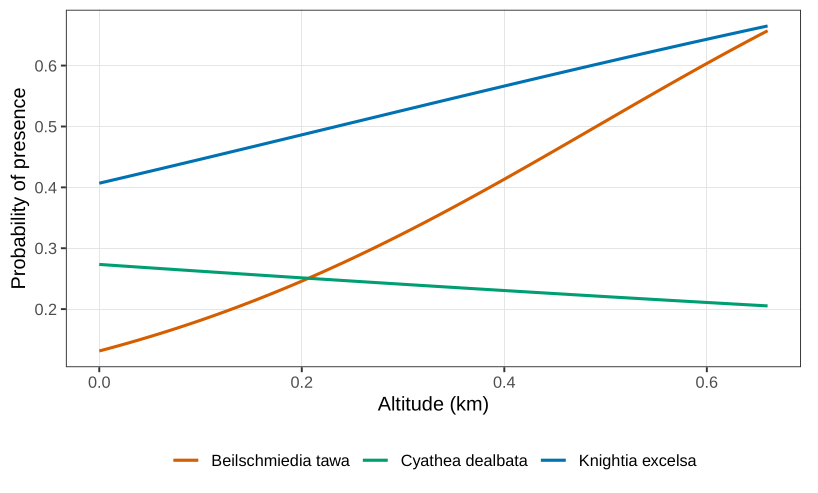
loglinb3. Beilschmiedia is uncommon at sea level and climbs. Cyathea is almost flat. Knightia sits between them.
At sea level the log-odds of Cyathea are -0.977, so the probability is \exp(-0.977)/(1+\exp(-0.977))\approx 0.27. Each extra kilometre of altitude multiplies those odds by \exp(-0.570)=0.57, but a sandwich z of -0.70 is not a claim of an altitude effect for Cyathea. Beilschmiedia is uncommon at sea level, probability \exp(-1.890)/(1+\exp(-1.890))\approx 0.13, and it prefers height: \exp(3.85)\approx 47 times the odds per kilometre, with sandwich z=4.42. In Figure 1 that climb is the steep curve. Knightia is the intermediate case, and its altitude slope is not detected (z=1.36). The naive and sandwich standard errors are the same order of magnitude, which is consistent with a working model that is not wildly wrong. It is still a pairwise model on a three-species hillside, so the sandwich column is the one to trust, not because the odds ratios are correct, but because those standard errors do not need them to be.
The fitted probabilities at the first location, the eight possible presence patterns of the three plants, start at 0.267 for “none of them”. Those eight probabilities are a joint distribution under the working model. They are not required for the slope estimates.
- From the Hunua table, compute the sea-level probability for Beilschmiedia tawa and the multiplicative change in its odds per kilometre of altitude. Use the sandwich z-statistic, not the naive one, when stating whether altitude is detected.
What links here
No other page links here yet.