Reliability
Part of Probability · 7 questions on this topic · What links here
Reliability
| Part | Probability |
| Chapter | 7 of 7 in this part |
| Previous | Markov chains |
| Questions | 7 |
| Definitions | Structure function · Reliability function · Survival function · Hazard rate · Weibull distribution |
| Figures | 3 |
Reliability is the probability that a system of unreliable components is working. The structure function says which patterns of working components make the system work. Once the component states are random, the reliability function turns those patterns into a probability. Adding time turns the same function into a lifetime distribution.
Component lifetimes in this chapter are exponential, Weibull, or another law from Random variables and distributions. The exponential and gamma formulas, means and variances are on the common distributions page. The Weibull law is not on that sheet, so it is recorded here.
Structure
Each of n components is either working or failed. Encode that by x_i\in\{0,1\}, with x_i=1 when component i works. The system itself is working or failed, and in the model used here the system state is a function of the component states alone.
Definition 1 (Structure function) The structure function \varphi:\{0,1\}^n\to\{0,1\} equals 1 when the system works and 0 when it has failed. A system is monotone when \mathbf{x}\le\mathbf{y} implies \varphi(\mathbf{x})\le\varphi(\mathbf{y}): repairing a component cannot cause a failure.
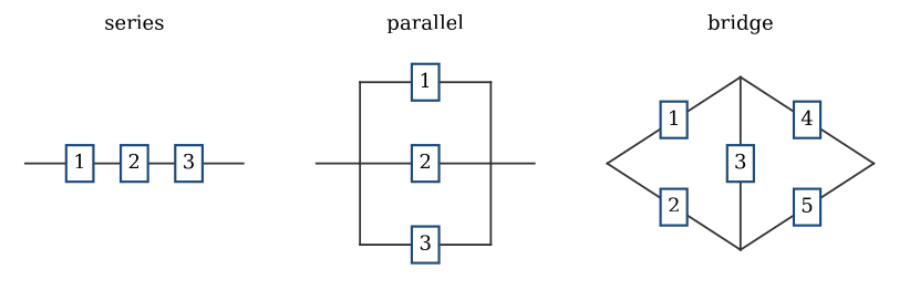
A series system works only when every component works, so \varphi(\mathbf{x})=\prod_{i=1}^n x_i. A parallel system works when at least one component works, so \varphi(\mathbf{x})=1-\prod_{i=1}^n(1-x_i). A k-out-of-n system works when at least k components work, so \varphi(\mathbf{x})=1 if \sum_i x_i\ge k and 0 otherwise. Series is n-out-of-n. Parallel is 1-out-of-n.
A system built by nesting series and parallel pieces can be reduced one module at a time. If component 1 stands in series with a parallel module whose two branches are the series pairs (x_2,x_3) and (x_4,x_5), then
\varphi(\mathbf{x})=x_1\bigl(1-(1-x_2 x_3)(1-x_4 x_5)\bigr).
A bridge cannot be drawn as a pure series–parallel graph. Label the two side paths 1–4 and 2–5, and let 3 be the cross link. Pivoting on the cross link splits the structure in two:
\varphi(\mathbf{x})=x_3 z_1+(1-x_3)z_2.
When the cross link works, the left side is joined to the right side, so z_1=\bigl(1-(1-x_1)(1-x_2)\bigr)\bigl(1-(1-x_4)(1-x_5)\bigr). When it has failed, the two side paths are separate, so z_2=1-(1-x_1 x_4)(1-x_2 x_5).
A minimal path set is a set of components whose working is enough to make the system work, and no proper subset is enough. A minimal cut set is a set whose failure is enough to make the system fail, and no proper subset is enough. For the bridge the minimal path sets are \{1,4\}, \{2,5\}, \{1,3,5\} and \{2,3,4\}, and the minimal cut sets are \{1,2\}, \{4,5\}, \{1,3,5\} and \{2,3,4\}.
If P_1,\ldots,P_m are the minimal path sets and K_1,\ldots,K_k the minimal cut sets of a monotone system, then
\varphi(\mathbf{x})=1-\prod_{j=1}^m\Bigl(1-\prod_{i\in P_j} x_i\Bigr) =\prod_{j=1}^k\Bigl(1-\prod_{i\in K_j}(1-x_i)\Bigr).
The first expression says the system works when at least one minimal path is entirely working. The second says it works when every minimal cut still has a working component. Expanding either expression, and using x_i^2=x_i, produces a multilinear polynomial in the x_i.
The reliability function
Now let the component state X_i be random, with \mathbb{P}(X_i=1)=p_i and \mathbb{P}(X_i=0)=1-p_i. The system works with probability \mathbb{P}(\varphi(\mathbf{X})=1)=\mathbb{E}\varphi(\mathbf{X}). In general this probability is not a function of the p_i alone, because the components may be dependent. From here on the component states are assumed independent.
Definition 2 (Reliability function) Under independent component states, the reliability function is r(\mathbf{p})=\mathbb{P}(\varphi(\mathbf{X})=1), a function of the vector \mathbf{p}=(p_1,\ldots,p_n).
Independence makes r the structure polynomial with each x_i replaced by p_i, but only after the polynomial has been written so that no x_i appears to a power higher than one. Substituting into \varphi(\mathbf{x})=\prod x_i is legal, and gives r(\mathbf{p})=\prod p_i for a series system. For a parallel system, r(\mathbf{p})=1-\prod(1-p_i). For a k-out-of-n system with a common reliability p,
r(p)=\sum_{i=k}^n \binom{n}{i} p^i(1-p)^{n-i},
the upper tail of the binomial distribution. The algebraic expression for r can look like \varphi, but the two functions have different domains: \varphi eats binary vectors and r eats probabilities.
For the bridge, expanding the path formula and reducing squares gives
\begin{align*} r(\mathbf{p}) &= p_1 p_4+p_2 p_5+p_1 p_3 p_5+p_2 p_3 p_4 \\ &\quad -p_1 p_2 p_3 p_5-p_1 p_2 p_4 p_5-p_1 p_3 p_4 p_5-p_1 p_2 p_3 p_4 \\ &\quad -p_2 p_3 p_4 p_5+2 p_1 p_2 p_3 p_4 p_5. \end{align*}
For a large system the exact polynomial can be out of reach. If E_j is the event that every component in the minimal cut K_j has failed, then r(\mathbf{p})=1-\mathbb{P}(\bigcup_j E_j). Inclusion–exclusion expands the union. Truncating after the first term, \sum_j \mathbb{P}(E_j), is the rare-event approximation, and it is accurate when every p_i is close to 1 and the cuts are unlikely.
Example 1 (A bridge of reliable links) Each of the five components of the bridge works with probability p=0.9, independently.
Question. Find the reliability of the bridge exactly, and by the rare-event approximation.
Solution. With every p_i=p the polynomial above collapses to
r(p)=2p^2+2p^3-5p^4+2p^5,
so r(0.9)=1.62+1.458-3.2805+1.181=0.9785. For the approximation, the minimal cuts \{1,2\} and \{4,5\} each fail with probability 0.1^2=0.01, and \{1,3,5\} and \{2,3,4\} each with 0.1^3=0.001, so
r\approx1-(0.01+0.01+0.001+0.001)=0.978.
The approximation is good to three decimal places, because with reliable components two cuts almost never fail together. It also shows where the risk is: the two-component cuts at each end contribute ten times as much as the three-component cuts through the cross link. For comparison, two parallel series paths without the cross link have reliability 1-(1-0.81)^2=0.964, so the link removes about 40% of the failure probability.
Lifetimes
Give each component a lifetime T_i with distribution function F_i, and assume the lifetimes are independent. The component is working at time t when T_i>t, so its reliability at time t is 1-F_i(t). The system lifetime T satisfies
\mathbb{P}(T\le t)=1-r\bigl(1-F_1(t),\ldots,1-F_n(t)\bigr).
A string of bulbs in series fails at the first bulb failure. If 20 bulbs have independent exponential lifetimes with mean 1000 hours, the rate of each bulb is 1/1000, the minimum is exponential with rate 20/1000, and the expected life of the string is 50 hours. That is the series formula r(\mathbf{p})=\prod p_i with p_i=e^{-t/1000}.
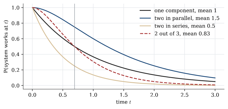
Example 2 (Mean lifetimes of redundant systems) Components have independent exponential lifetimes with rate \lambda, so each has mean 1/\lambda.
Question. Compare the mean lifetimes of one component, two components in parallel, and a 2-out-of-3 system.
Solution. The mean is the integral of the survival function. With q(t)=e^{-\lambda t}, two in parallel survive with probability 1-(1-q)^2=2q-q^2, so
\mathbb{E} T=\int_0^\infty\bigl(2e^{-\lambda t}-e^{-2\lambda t}\bigr)\,\mathrm{d} t=\frac2\lambda-\frac1{2\lambda}=\frac3{2\lambda}.
A 2-out-of-3 system survives with probability 3q^2(1-q)+q^3=3q^2-2q^3, so
\mathbb{E} T=\int_0^\infty\bigl(3e^{-2\lambda t}-2e^{-3\lambda t}\bigr)\,\mathrm{d} t=\frac3{2\lambda}-\frac2{3\lambda}=\frac5{6\lambda}.
The 2-out-of-3 system lives on average less long than a single component, even though at p=0.9 its reliability, 0.972, beats a single component’s 0.9. Redundancy helps while components are likely to be working, early on, and hurts later, when the system needs two survivors out of a shrinking pool. A reliability at one time and a mean lifetime answer different questions.
Hazard and the Weibull law
Definition 3 (Survival function) The survival function of a lifetime T with distribution function F is R(t)=\mathbb{P}(T>t)=1-F(t) for t\ge 0.
For a non-negative random variable the expectation is the integral of the survival function, \mathbb{E} T=\int_0^{\infty} R(t)\,\,\mathrm{d} t, when the integral exists. The argument is integration by parts, or Fubini’s theorem applied to \mathbb{E} T=\mathbb{E}\int_0^{T} 1\,\,\mathrm{d} t=\int_0^{\infty}\mathbb{P}(T>t)\,\,\mathrm{d} t. The mean time to failure is this expectation.
Definition 4 (Hazard rate) If T has density f and survival function R, the hazard rate is h(t)=f(t)/R(t) for t with R(t)>0.
For small \varepsilon>0, \mathbb{P}(T\in[t,t+\varepsilon]\mid T>t)\approx \varepsilon\, h(t). The hazard is the instantaneous failure rate among components still alive at t. An increasing hazard is an ageing component. A decreasing hazard is one that becomes less prone to failure as time passes, which can happen when weak individuals fail early. The hazard determines the survival function:
R(t)=\exp\Bigl(-\int_0^t h(u)\,\,\mathrm{d} u\Bigr).
The exponential distribution with rate \lambda has constant hazard \lambda. Assuming an exponential lifetime is assuming that the component does not age. That is the same fact as the memoryless property.
Definition 5 (Weibull distribution) A lifetime T is Weibull with shape \beta>0 and rate \lambda>0 when its density is \lambda\beta\,(\lambda t)^{\beta-1}\exp(-(\lambda t)^\beta) for t>0. The survival function is \exp(-(\lambda t)^\beta), the distribution function is 1 minus that survival function, and
\mathbb{E} T=\frac{\Gamma(1+1/\beta)}{\lambda}.
The shape \beta=1 is the exponential distribution with rate \lambda.
The Weibull hazard is h(t)=\lambda\beta(\lambda t)^{\beta-1}. It increases when \beta>1 and decreases when \beta<1. Shape is the ageing parameter. Rate sets the time scale.
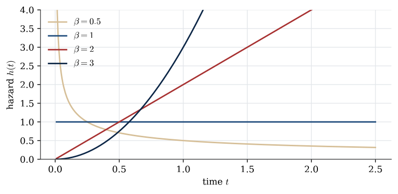
A Weibull lifetime with shape \beta=2 and rate \lambda=0.001 per hour has mean \Gamma(1.5)/0.001=886 hours, and its hazard grows linearly in time: at 1000 hours it is 2\times0.001\times1=0.002 per hour, twice what it was at 500 hours.
Write the binary function that says when the system works, reduce it to a multilinear polynomial, and under independence replace each component indicator by its reliability. Put survival probabilities in place of those reliabilities to get the lifetime of a system that is not repaired.
Questions on this topic
Open a question to attempt it. Its worked answer is folded away at the bottom of the page.
What links here
Pages (3)
- Random experiments and probability — via Reliability, parallel system
- Random variables and distributions — via failure rate, reliability
- Functions of random variables and limit theorems — via survival function
Questions and answers (6)
See also
- Articles from this chapter: Structure function · Reliability function · Survival function · Hazard rate · Weibull distribution
- All probability chapters
- Glossary and index
- Distribution sheet and formula lookup