Markov chains
Part of Probability · 6 questions on this topic · What links here
Markov chains
| Part | Probability |
| Chapter | 6 of 7 in this part |
| Previous | Functions of random variables and limit theorems |
| Next | Reliability |
| Questions | 6 |
| Definitions | Finite-state Markov chain |
| Results | Limiting distribution |
| Figures | 3 |
A Markov chain is a random process with a short memory: the next state depends on the past only through the present state. On a finite set of states the whole process is a transition matrix. Powers of that matrix give the distribution after many steps, and for a chain that can reach every state and is not periodic, those powers settle on a single row vector, the limiting distribution.
Using a chain as a device for sampling from a target distribution is a different construction. That use, including the Gibbs sampler and Metropolis–Hastings, is on Markov chains, Gibbs sampling, and Metropolis–Hastings. The vector called a limiting distribution here is called a stationary distribution there. This chapter stays with the process itself.
The Markov property
Definition 1 (Finite-state Markov chain) Let E be a finite set of states and let X_0,X_1,X_2,\ldots take values in E. The process is a Markov chain when, for every n and every choice of states,
\mathbb{P}(X_{n+1}=j\mid X_n=i, X_{n-1}=i_{n-1},\ldots,X_0=i_0)=\mathbb{P}(X_{n+1}=j\mid X_n=i).
It is time-homogeneous when the right-hand side does not depend on n. The transition matrix P then has entries P_{ij}=\mathbb{P}(X_{n+1}=j\mid X_n=i).
Each row of P is a probability distribution: the entries are non-negative and sum to 1. If the row vector \boldsymbol\pi^{(0)} is the distribution of X_0, the distribution of X_n is \boldsymbol\pi^{(0)} P^n. The Chapman–Kolmogorov equations are the matrix product P^{m+n}=P^m P^n: the way to be at j after m+n steps is to be somewhere after m steps and then travel for n more.
A path of length n has probability equal to the product of the n transition probabilities along it, times the probability of the starting state. That product is the Markov property written out by the chain rule. A chain is conveniently drawn as a transition graph: one node per state, and an arrow from i to j, labelled P_{ij}, whenever P_{ij}>0.
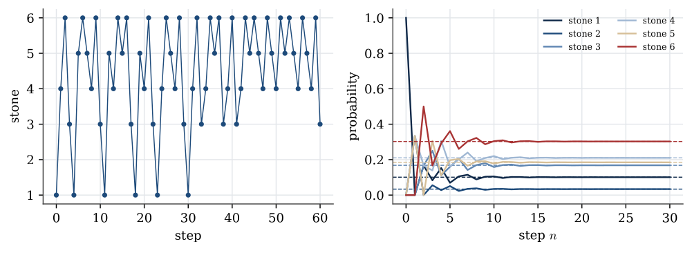
Example 1 (Six stepping stones) A frog hops between six stepping stones. From each stone it jumps to one of the stones joined to it, choosing uniformly among them, except that from stone 4 it always goes to stone 6. The transition matrix, with rows and columns in the order of the stones, is
P=\begin{pmatrix} 0&1/3&0&1/3&1/3&0\\ 1/2&0&1/2&0&0&0\\ 1/2&0&0&1/2&0&0\\ 0&0&0&0&0&1\\ 0&0&0&1/2&0&1/2\\ 0&0&1/2&0&1/2&0 \end{pmatrix}.
Question. Starting on stone 1, find the distribution after two steps, and the long-run proportion of time spent on each stone.
Solution. The distribution after two steps is the first row of P^2:
(1/6,\ 0,\ 1/6,\ 1/6,\ 0,\ 1/2).
For example, stone 6 is reached in two steps through stone 4 or stone 5, with probability \tfrac13\cdot1+\tfrac13\cdot\tfrac12=\tfrac12. Stones 2 and 5 cannot be reached from stone 1 in exactly two steps. After ten steps the probability of being back on stone 1 is 0.1049, and by n=100 every row of P^n agrees to four decimal places.
The chain is irreducible, and it is aperiodic because it can return to stone 1 in both 2 and 3 steps, which have greatest common divisor 1. Solving \boldsymbol\pi=\boldsymbol\pi P with \sum_j\pi_j=1 gives
\boldsymbol\pi=\frac1{119}(12,\ 4,\ 20,\ 25,\ 22,\ 36)=(0.101,\ 0.034,\ 0.168,\ 0.210,\ 0.185,\ 0.303).
The first equation, \pi_2=\pi_1/3, says that stone 2 is entered only from stone 1, a third of the time. In the long run the frog spends 30% of its time on stone 6 and only 3% on stone 2, whichever stone it started from.
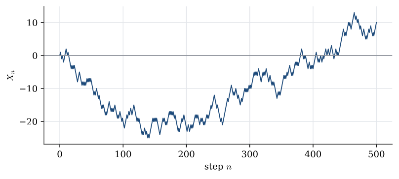
A random walk on the integers, moving one step right with probability p and one step left with probability q=1-p, is the same definition on a countably infinite state space. The one-step matrix is no longer a finite array, but the n-step probabilities are binomial: after n steps the displacement is 2K-n if K\sim\operatorname{Bin}(n,p) is the number of steps to the right.
States i and j communicate when each can be reached from the other with positive probability in some number of steps. A chain on a finite set is irreducible when every pair communicates. A state is periodic with period d>1 when returns are possible only at multiples of d; otherwise it is aperiodic. In an irreducible chain every state has the same period.
Simulation
One step of a finite-state chain is a discrete draw from the row P_{i,\cdot}, which is the discrete inverse-transform method applied to that row. A path is the iteration: given X_n=i, draw X_{n+1} from row i, independently of the earlier past.
A random walk on the integers is even simpler. Draw independent steps \xi_k\in\{-1,+1\} with \mathbb{P}(\xi_k=+1)=p, and set X_n=X_0+\xi_1+\cdots+\xi_n. The partial-sum representation makes the binomial count of rightward steps obvious.
The limiting distribution
Theorem 1 (Limiting distribution) Suppose P is the transition matrix of an irreducible aperiodic chain on a finite set. Then there is a unique probability row vector \boldsymbol\pi with \boldsymbol\pi=\boldsymbol\pi P, and for every start i and every state j,
\lim_{n\to\infty}(P^n)_{ij}=\pi_j.
Every row of P^n converges to \boldsymbol\pi. The equations \boldsymbol\pi=\boldsymbol\pi P together with \sum_j \pi_j=1 determine \boldsymbol\pi.
The vector \boldsymbol\pi is the distribution that is unchanged by one more step. Irreducibility keeps the chain from getting stuck in a subset of states. Aperiodicity keeps the distribution from oscillating between two or more patterns; a deterministic two-cycle is irreducible and has no limiting distribution, even though it has a stationary one.
On a small state space the linear system (P^\top-I)\boldsymbol\pi^\top=\mathbf{0} is solved directly, and the solution is scaled so that its entries sum to 1. A null-space routine does the same arithmetic. For the stepping stones this is the vector found above.
Example 2 (A two-state weather chain) Each day is dry or wet. A dry day is followed by a dry day with probability 0.8, and a wet day by a wet day with probability 0.6.
Question. Find the limiting distribution, and the probability that it is dry two days after a wet day.
Solution. With the states in the order dry, wet,
P=\begin{pmatrix}0.8&0.2\\0.4&0.6\end{pmatrix}.
The balance equation for the dry state is \pi_1=0.8\pi_1+0.4\pi_2, so 0.2\pi_1=0.4\pi_2 and \pi_1=2\pi_2. With \pi_1+\pi_2=1, \boldsymbol\pi=(2/3,1/3): in the long run two days in three are dry. Two days after a wet day, the probability of a dry day is the (wet, dry) entry of P^2,
0.4\times0.8+0.6\times0.4=0.56.
For any two-state chain with switching probabilities a (dry to wet) and b (wet to dry), the limit is (b,a)/(a+b), and P^n approaches it geometrically fast, at rate (1-a-b)^n. Here 1-a-b=0.4, so after a week the starting state has almost no influence.
The limiting distribution also describes a single long path. For an irreducible chain on a finite set, the fraction of the first n steps spent in state j converges to \pi_j with probability one, whatever the start. This is a law of large numbers for a dependent sequence. It is what justifies estimating \pi by running one long simulation and counting visits, and it is the fact that Markov chain Monte Carlo rests on.
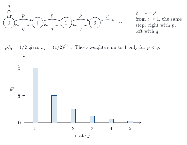
A random walk on the non-negative integers, with reflection at 0, shows when a limit exists on an infinite space. From 0 the walk steps to 1 with probability p and stays with probability q=1-p. From j\ge 1 it steps to j+1 with probability p and to j-1 with probability q. The balance equations \boldsymbol\pi=\boldsymbol\pi P give \pi_j=(p/q)^j \pi_0 for j\ge 0. These numbers can be scaled to sum to 1 if and only if p<q, in which case \pi_0=1-p/q and \pi_j=(1-p/q)(p/q)^j. If p\ge q the walk drifts to infinity and no probability vector satisfies the balance equations. The chain still has the Markov property. It simply has no limiting distribution.
The next state is drawn from a row of P that depends only on the current state. After many steps an irreducible aperiodic finite chain forgets where it started, and the probability of each state settles on the unique row vector \boldsymbol\pi=\boldsymbol\pi P.
Questions on this topic
Open a question to attempt it. Its worked answer is folded away at the bottom of the page.
What links here
Pages (1)
- Markov chains, Gibbs sampling, and Metropolis–Hastings — via transition matrix
Questions and answers (3)
See also
- Articles from this chapter: Finite-state Markov chain · Limiting distribution
- All probability chapters
- Glossary and index
- Distribution sheet and formula lookup