Metropolis–Hastings update
Definition taught in Markov chains, Gibbs sampling, and Metropolis–Hastings, part of Bayesian statistics
Metropolis–Hastings update
| Type | Definition |
| Taught in | Markov chains, Gibbs sampling, and Metropolis–Hastings |
| Part | Bayesian statistics |
| Properties | 2 |
| Worked examples | 3 |
| Questions using it | 15 |
Let \pi(x) be a target density known only up to proportionality. Given X_t=x:
propose Y=y from a proposal density q(y\mid x);
calculate r(x,y) from Equation (4) in Markov chains, Gibbs sampling, and Metropolis–Hastings and put a(x,y)=\min\{1,r(x,y)\};
draw U\sim\operatorname{Unif}(0,1) and set
X_{t+1}= \begin{cases} y,&U\leq a(x,y),\\ x,&U>a(x,y). \end{cases}
If \pi(x)=f(x)/C for unknown C, then
\frac{\pi(y)}{\pi(x)} =\frac{f(y)/C}{f(x)/C} =\frac{f(y)}{f(x)},
so the normalising constant cancels.
Properties
Metropolis–Hastings invariance
Main article: Metropolis–Hastings invariance
The Metropolis–Hastings transition defined by Equation (5) in Markov chains, Gibbs sampling, and Metropolis–Hastings satisfies detailed balance with respect to \pi. Consequently, \pi is stationary.
Warm-up is not a convergence proof
Main article: Warm-up is not a convergence proof
The chain should be initialised in a plausible region when one is available. A start many standard deviations from the typical set can require a long time to return, while a start at the mean of a separated mixture can lie in a low-density gap. Multiple dispersed chains help reveal failure to explore all modes; they do not repair it automatically.
Discarding early draws is called warm-up or burn-in. It limits dependence on the chosen initial state, but it is not a proof of convergence. Strong posterior correlation produces staircase-like Gibbs paths and high autocorrelation. Separated modes are harder still because a coordinate-wise move may have to cross a low-density barrier.
Thinning by retaining every kth draw reduces storage and visible serial dependence, but usually throws away usable information. Unless storage or an expensive downstream calculation is the constraint, retain all post-warm-up draws and quantify their effective sample size. Posterior means, probabilities, and equal-tailed intervals are computed from those draws; a continuous MAP is found by optimisation, not by asking which simulated value occurred most often.
Examples
Q5. Random-walk Metropolis-Hastings
Question page: Q5. Random-walk Metropolis-Hastings
Let the target density be \pi(x)\propto x^2e^{-x}, \qquad x>0. We wish to sample from \pi using a random-walk Metropolis-Hastings algorithm with proposal Y\mid X^{(t-1)}=x\sim\mathcal{N}(x,\sigma^2), where \sigma>0 is fixed.
(a) [3 marks] Show that the Metropolis-Hastings acceptance probability is \alpha(x,y) = \begin{cases} \displaystyle \min\left\{ \left(\frac{y}{x}\right)^2 e^{-(y-x)},1 \right\}, & y>0,\\[1.2em] 0, & y\leq0. \end{cases} Explain why the proposal-density terms cancel.
(b) [2 marks] Calculate the acceptance probability for each proposed move. You may leave your answers in exact exponential form.
1. Current state x=2, proposed state y=3.
2. Current state x=3, proposed state y=2.
(c) [3 marks] Write pseudocode for a random-walk Metropolis-Hastings sampler generating T observations from the target distribution. Begin from a valid initial value x^{(0)}>0.
(d) [1 mark] Explain why the unknown normalising constant of \pi(x) is not required.
(e) [2 marks] Are the sampled values X^{(1)},X^{(2)},\ldots,X^{(T)} independent? Briefly explain.
(f) [2 marks] Explain what is likely to happen if:
1. \sigma is extremely small;
2. \sigma is extremely large.
Definitions. Write q(y\mid x) for the density of a proposal y from current state x, and \alpha(x,y) for its acceptance probability. The target kernel is x^2e^{-x} on x>0 and zero elsewhere. N(x,\sigma^2) uses variance \sigma^2, held fixed and positive throughout the run; start with x^{(0)}>0.
As a recognition check, \pi(x)\propto x^{3-1}e^{-1\cdot x}, \qquad x>0, is the kernel of a \operatorname{Gamma}(3,1) distribution under the shape-rate convention. The exercise nevertheless asks us to construct a Metropolis-Hastings sampler for this target.
(a) Acceptance probability
For a proposal density q(y\mid x), the Metropolis-Hastings acceptance probability is \alpha(x,y) =\min\left\{ \frac{\pi(y)q(x\mid y)}{\pi(x)q(y\mid x)},1 \right\}. The normal random-walk proposal is symmetric because q(y\mid x) =\frac{1}{\sqrt{2\pi\sigma^2}} \exp\left[-\frac{(y-x)^2}{2\sigma^2}\right] =q(x\mid y). The proposal-density terms therefore cancel. If y>0, the target-density ratio is \frac{\pi(y)}{\pi(x)} =\frac{y^2e^{-y}}{x^2e^{-x}} =\left(\frac{y}{x}\right)^2e^{-(y-x)}. If y\leq0, then y is outside the support of the target and the proposal must be rejected. Hence \boxed{ \alpha(x,y) = \begin{cases} \displaystyle \min\left\{ \left(\frac{y}{x}\right)^2e^{-(y-x)},1 \right\}, & y>0,\\[1.2em] 0, & y\leq0. \end{cases} }
(b) Acceptance probabilities for the two moves
1. For x=2 and y=3, \alpha(2,3) =\min\left\{\left(\frac32\right)^2e^{-1},1\right\} =\boxed{\frac{9}{4e}\approx0.828}, since 9/(4e)<1. Thus the move is accepted with probability about 82.8\%.
2. For x=3 and y=2, \alpha(3,2) =\min\left\{\left(\frac23\right)^2e,1\right\} =\min\left\{\frac{4e}{9},1\right\} =\boxed{1}, since 4e/9>1. This move goes to a point of higher target density and is always accepted.
This illustrates the basic Metropolis rule: moves to higher target density are accepted automatically, while moves to lower target density may still be accepted with positive probability.
(c) Random-walk Metropolis-Hastings pseudocode
Choose an initial state x^{(0)}>0. For t=1,2,\ldots,T:
1. Generate a proposal Y\sim\mathcal{N}\bigl(x^{(t-1)},\sigma^2\bigr).
2. Calculate a= \begin{cases} \displaystyle \min\left\{ \left(\frac{Y}{x^{(t-1)}}\right)^2 e^{-(Y-x^{(t-1)})},1 \right\}, & Y>0,\\[1.2em] 0, & Y\leq0. \end{cases}
3. Independently generate U\sim\operatorname{Unif}(0,1).
4. Set X^{(t)}= \begin{cases} Y, & U\leq a,\\ X^{(t-1)}, & U>a. \end{cases}
5. Store X^{(t)}.
A rejection does not mean that nothing is recorded: the chain stores the current value again, so X^{(t)}=X^{(t-1)}. After a suitable burn-in, the stored values are approximately distributed according to \pi.
(d) Unknown normalising constant
If \pi(x)=\widetilde{\pi}(x)/C, then \frac{\pi(y)}{\pi(x)} =\frac{\widetilde{\pi}(y)/C}{\widetilde{\pi}(x)/C} =\frac{\widetilde{\pi}(y)}{\widetilde{\pi}(x)}. Thus the same unknown constant appears in the numerator and denominator and cancels from the acceptance ratio. Metropolis-Hastings therefore requires the target only up to proportionality, which is especially useful for posterior distributions with an intractable marginal likelihood.
(e) Independence of the sampled values
No. Each proposal is generated from the previous state, and a rejected move gives X^{(t)}=X^{(t-1)}. The samples therefore form a Markov chain and are generally serially dependent, even after the chain has reached equilibrium. At equilibrium, each X^{(t)} has marginal distribution \pi, but having the correct marginal distribution does not imply independence.
(f) Effect of the proposal scale
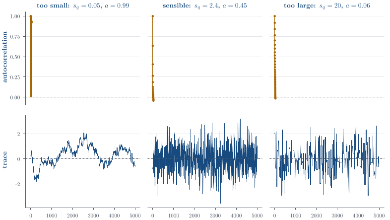
1. If \sigma is extremely small, proposals stay close to the current state and are usually accepted. However, the chain moves slowly through the target distribution, producing high autocorrelation and poor mixing.
2. If \sigma is extremely large, many proposals fall outside the support or in regions of very low target density. The acceptance rate becomes small, so the chain often repeats its current value and again mixes poorly.
Q10. Metropolis-Hastings with an asymmetric-proposal extension
A posterior density is known up to a normalising constant: p(\theta\mid{\boldsymbol{x}})\propto\theta^2e^{-\theta}, \qquad \theta>0. From the current state \theta^{(t)}>0, propose \theta^*=\theta^{(t)}+\varepsilon, \qquad \varepsilon\sim\mathcal{N}(0,s^2), where s>0 is fixed.
(a) Derive the acceptance probability, including the case \theta^*\leq0. Explain why the unknown normalising constant is not needed. [3 marks]
(b) Give pseudocode for one iteration, including the acceptance decision and the next state after rejection. [3 marks]
(c) One run uses a very small s and accepts almost every proposal. Another uses a very large s and accepts very few. Explain why either run may be inefficient. [2 marks]
(d) If the proposal density were not symmetric, what additional factor would be required in the acceptance ratio? Define its numerator and denominator. [2 marks]
Definitions. The target is proportional to \theta^2e^{-\theta} on \theta>0 and is zero otherwise. Let q(\theta^*\mid\theta) be the proposal density, \alpha(\theta,\theta^*) the acceptance probability, and (t) the iteration index. The proposal N(\theta,s^2) has variance s^2>0, fixed across states and iterations; the current state must lie in the target support.
The target density has kernel \pi(\theta)\propto \theta^2e^{-\theta}, \qquad \theta>0.
(a) Acceptance probability
For a random-walk proposal \theta^*\mid\theta^{(t)}\sim N\left(\theta^{(t)},s^2\right), the proposal is symmetric: q(\theta^*\mid\theta^{(t)}) =q(\theta^{(t)}\mid\theta^*). Consequently, the proposal-density terms cancel from the Metropolis–Hastings ratio. If \theta^*>0, \begin{aligned} \alpha\left(\theta^{(t)},\theta^*\right) &= \min\left\{ \frac{\pi(\theta^*)}{\pi(\theta^{(t)})},1 \right\}\\ &= \boxed{ \min\left\{ \left(\frac{\theta^*}{\theta^{(t)}}\right)^2 \exp\left[-\left(\theta^*-\theta^{(t)}\right)\right], 1 \right\}. } \end{aligned} If \theta^*\leq 0, then \pi(\theta^*)=0, so the proposal is rejected and \alpha=0.
(b) Normalising constant
The unknown normalising constant appears in both the numerator and denominator of the target-density ratio and therefore cancels. Only the target kernel is needed.
(c) One sampler iteration
One iteration of the algorithm is:
1. Generate a proposal \theta^*\sim N\left(\theta^{(t)},s^2\right).
2. Calculate \alpha(\theta^{(t)},\theta^*) as above.
3. Generate U\sim\operatorname{Uniform}(0,1).
4. Set \theta^{(t+1)}= \begin{cases} \theta^*, & U\leq\alpha(\theta^{(t)},\theta^*),\\ \theta^{(t)}, & U>\alpha(\theta^{(t)},\theta^*). \end{cases}
(d) Proposal scale
If s is extremely small, proposals remain close to the current state and the acceptance rate will usually be high. However, the chain moves only in small steps, producing high autocorrelation and slow exploration.
If s is extremely large, many proposals will be negative or will fall in regions where the target density is very small. Most will be rejected, so the chain will repeatedly remain at the same state and again mix slowly.
(e) Asymmetric proposals
For an asymmetric proposal, the proposal terms do not cancel. The acceptance probability becomes \boxed{ \alpha(\theta,\theta^*) = \min\left\{ \frac{\pi(\theta^*)q(\theta\mid\theta^*)} {\pi(\theta)q(\theta^*\mid\theta)}, 1 \right\}. } The additional factor is therefore \boxed{ \frac{q(\theta\mid\theta^*)}{q(\theta^*\mid\theta)}, } that is, the reverse-proposal density divided by the forward-proposal density.
Metropolis–Hastings for the logit-normal posterior
Question page: Metropolis–Hastings for the logit-normal posterior
Use the posterior kernel in the logit-normal prior exercise.
For n=40 and x=16, use a Metropolis–Hastings algorithm to retain 10{,}000 draws after a burn-in of 1{,}000. Plot a kernel-density estimate and describe it.
Estimate the posterior mean, compare it with the prior mean, and explain how the data have changed the distribution.
Estimate and interpret an equal-tailed 95\% credible interval.
Repeat the numerical summaries for n=400 and x=160. Explain why ten times as much data changes the spread far more than the centre.
Question. For 0<\theta<1, take the posterior target
\pi(\theta\mid x,n)\propto \theta^{x-1}(1-\theta)^{n-x-1} \exp\!\left[-\frac12\{\operatorname{logit}(\theta)-1\}^2\right].
For n=40 and x=16, use a Metropolis–Hastings algorithm to retain 10{,}000 draws after a burn-in of 1{,}000. Plot a kernel-density estimate and describe it.
Estimate the posterior mean, compare it with the prior mean, and explain how the data have changed the distribution.
Estimate and interpret an equal-tailed 95\% credible interval.
Repeat the numerical summaries for n=400 and x=160. Explain why ten times as much data changes the spread far more than the centre.
Solution. For numerical stability define the log of the unnormalised target by
\ell(\theta;x,n) =(x-1)\log\theta+(n-x-1)\log(1-\theta) -\frac12\{\operatorname{logit}(\theta)-1\}^2.
Use an independent \operatorname{Beta}(A,B) proposal with density g. Since this is not a random walk, the proposal terms do not cancel. For current state \theta and proposal y, \begin{align*} r(\theta,y) &=\frac{\pi(y)g(\theta)}{\pi(\theta)g(y)},\\ \log r(\theta,y) &=\ell(y;x,n)-\ell(\theta;x,n) +\log g(\theta)-\log g(y),\\ a(\theta,y)&=\min\{1,r(\theta,y)\}. \end{align*} The following implementation uses \operatorname{Beta}(4,6) for (x,n)=(16,40) and \operatorname{Beta}(40,60) for (160,400).
log_posterior <- function(theta, x, n) {
  ifelse(theta <= 0 | theta >= 1, -Inf,
         (x - 1) * log(theta) +
         (n - x - 1) * log1p(-theta) -
         0.5 * (qlogis(theta) - 1)^2)
}
independent_mh <- function(x, n, A, B, keep = 10000, burn = 1000) {
  total <- keep + burn
  out <- numeric(total)
  out[1] <- x / n
  for (t in 2:total) {
    proposed <- rbeta(1, A, B)
    log_ratio <-
      log_posterior(proposed, x, n) -
      log_posterior(out[t - 1], x, n) +
      dbeta(out[t - 1], A, B, log = TRUE) -
      dbeta(proposed, A, B, log = TRUE)
    if (log(runif(1)) < min(0, log_ratio)) {
      out[t] <- proposed
    } else {
      out[t] <- out[t - 1]
    }
  }
  out[(burn + 1):total]
}
set.seed(3500)
draw40  <- independent_mh(16,  40,  4,  6)
draw400 <- independent_mh(160, 400, 40, 60)
mean(draw40)
quantile(draw40, c(0.025, 0.975))
mean(draw400)
quantile(draw400, c(0.025, 0.975))
plot(density(draw40, from = 0, to = 1),
     xlab = expression(theta), main = "n = 40")
For the displayed seed, the n=40 run gives
\widehat{\mathbb{E}(\theta\mid x)}=0.432, \qquad \text{$95\%$ interval }(0.294,0.578).
Direct numerical integration gives 0.4320 and (0.291,0.579), so the Monte Carlo discrepancy is of the expected size. The prior mean is approximately 0.6967: observing only 16/40=0.4 heads moves the posterior sharply towards 0.4 and makes it appreciably more concentrated. The interval means that, under the model and prior, the posterior probability that \theta lies between the reported endpoints is approximately 0.95.
For n=400 and x=160, the same seed gives
\widehat{\mathbb{E}(\theta\mid x)}=0.404, \qquad \text{$95\%$ interval }(0.355,0.453),
while numerical integration gives 0.4035 and (0.356,0.452). Both data sets have empirical proportion 0.4, so the centre changes little. The ten-fold increase in sample size makes the likelihood much more concentrated and leaves the prior with much less leverage.
The function dbeta in the Hastings ratio is essential: g is a proposal density. Replacing it by the distribution function pbeta changes the invariant distribution and produces incorrect posterior summaries.
Used in
- Taught in Markov chains, Gibbs sampling, and Metropolis–Hastings, where the derivation and examples are.
- Also used in Simulation · Markov chains · Exponential families and conjugacy · Hierarchical Bayes · Reference formulas and problem-solving workflow
- Questions that use it (15) — Metropolis–Hastings for the logit-normal posterior · Random-walk Metropolis for a correlated normal · An independent Gamma proposal · Q4 (answer) · Q5 · Q10 · Q19 · Q25 · Q26 (answer) · Q42 · Q50 · Q52 · Q59 (answer) · Question 9 · C14
- All 31 questions on Markov chains, Gibbs sampling, and Metropolis–Hastings
See also
Metropolis–Hastings invariance · Markov chain · Stationarity and detailed balance · Detailed balance implies stationarity · Systematic-scan Gibbs sampler · Warm-up is not a convergence proof