Analysis of variance examples
Part of Data analysis · 2 questions on this topic · What links here
Analysis of variance examples
| Part | Data analysis |
| Chapter | 6 of 9 in this part |
| Previous | Testing examples |
| Next | Regression examples |
| Questions | 2 |
| Definitions | Bonferroni correction · Interaction |
| Figures | 2 |
Analysis of variance compares the means of a quantitative response across the levels of one or more categorical factors. The model, the sum-of-squares split and the F distribution of the test statistic are in Analysis of variance. This page fits the models in R, reads the tables, checks the assumptions, and goes on to two factors and their interaction, which the inference chapter does not cover.
One factor
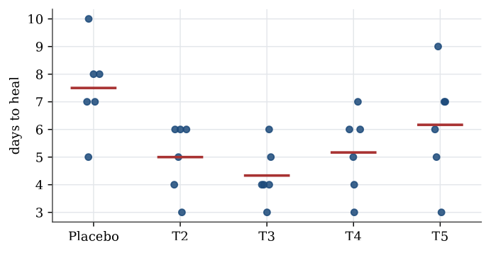
Example 1 (Five treatments for cold sores) Thirty patients with cold sores were assigned at random to five treatments, six to each; treatment 1 is a placebo. The days until the sore healed were
| Placebo | T2 | T3 | T4 | T5 |
|---|---|---|---|---|
| 5 | 4 | 6 | 7 | 9 |
| 8 | 6 | 4 | 4 | 3 |
| 7 | 6 | 4 | 6 | 5 |
| 7 | 3 | 5 | 6 | 7 |
| 10 | 5 | 4 | 3 | 7 |
| 8 | 6 | 3 | 5 | 6 |
Question. Do the treatments differ in mean healing time?
Solution. The table is not in standard form: for an analysis the healing times must be one column and the treatment a factor in another. stack does that.
x <- data.frame(Placebo = c(5, 8, 7, 7, 10, 8), T2 = c(4, 6, 6, 3, 5, 6),
                T3 = c(6, 4, 4, 5, 4, 3), T4 = c(7, 4, 6, 6, 3, 5),
                T5 = c(9, 3, 5, 7, 7, 6))
coldsore <- stack(x)
names(coldsore) <- c("times", "treatment")
tapply(coldsore$times, coldsore$treatment, mean)
# Placebo  T2    T3    T4    T5
#   7.500 5.000 4.333 5.167 6.167
coldsore.lm <- lm(times ~ treatment, data = coldsore)
anova(coldsore.lm)
#           Df Sum Sq Mean Sq F value  Pr(>F)
# treatment  4 36.467  9.1167  3.896 0.01359
# Residuals 25 58.500  2.3400
Under equal means F=3.90 would come from an F_{4,25} distribution, and the p-value is 0.014, so the treatments do differ. The placebo has the longest mean healing time, 7.5 days. The residual mean square, 2.34, estimates the common variance, so the within-group standard deviation is about 1.5 days.
Checking the model
The F test assumes independent normal errors with the same variance in every group. These are checked through the residuals, y_{ik}-\overline y_{i\cdot}: a plot of residuals against fitted values should show no pattern and similar spread in each group, and a normal quantile plot of the residuals should be close to a straight line.
plot(coldsore.lm, 1:2) # residuals against fitted values, and a normal Q-Q plotIndependence is not something a residual plot can verify. It comes from the design: here, from assigning treatments to separate patients at random.
Which groups differ?
A significant F says the means are not all equal; it does not say which ones differ. Comparing every pair with its own test at level \alpha inflates the chance of a false difference, since with five groups there are ten pairs.
Definition 1 (Bonferroni correction) To make m comparisons with a familywise error rate of at most \alpha, run each at level \alpha/m. Equivalently, multiply each p-value by m, capping at 1.
The correction works because the probability that at least one of m events occurs is at most the sum of their probabilities. It is simple and always valid, but conservative when m is large. Tukey intervals, built for all pairwise differences of means, are sharper. For the cold sores, Tukey’s method at familywise level 0.05 separates only one pair: placebo against treatment 3, with difference 3.17 days and 95% simultaneous interval (0.57,\ 5.76). The Bonferroni version agrees: the t statistic for that pair is 3.59, beyond the corrected critical value t_{25;\,1-0.05/20}=3.08, and no other pair passes.
TukeyHSD(aov(times ~ treatment, data = coldsore))
pairwise.t.test(coldsore$times, coldsore$treatment, p.adjust.method = "bonferroni")
The same question arises with unequal groups. Haemoglobin was measured for three forms of sickle-cell disease, in groups of 16 (HbSS), 15 (HbST) and 10 (HbSC). The analysis of variance gives a treatment sum of squares of 99.89 on 2 degrees of freedom and an error mean square of 1.00 on 38, so F=49.9 and the p-value is about 2.3\times10^{-11}. Bonferroni-corrected pairwise tests, with three comparisons each at level 0.05/3, then say which forms differ; the exercises work through them.
Two factors
Many experiments vary more than one factor. The model for two factors, with d_1 and d_2 levels and n_{ij} observations in cell (i,j), is
Y_{ijk}=\mu+\alpha_i+\beta_j+\gamma_{ij}+\varepsilon_{ijk}, \qquad \varepsilon_{ijk}\ \text{independent}\ \operatorname{N}(0,\sigma^2).
Here \mu is a baseline mean, \alpha_i and \beta_j are the main effects of the two factors, and \gamma_{ij} is their interaction. The parameters are not all identifiable as written; R fixes them by setting the effects of the first level of each factor to zero.
Definition 2 (Interaction) Two factors interact when the effect of one depends on the level of the other: the difference in mean response between two levels of the first factor is not the same at every level of the second. In the two-factor model, there is no interaction when every \gamma_{ij}=0.
An interaction plot draws the cell means of one factor against its levels, one line per level of the other factor. Parallel lines mean no interaction. With interaction present, the main effects on their own are hard to interpret: “the effect of fertilizer” is not a single number if it depends on the region.
The two-factor ANOVA table splits the total sum of squares into a part for each factor, a part for the interaction, and the error:
| Source | Df | F |
|---|---|---|
| Factor 1 | d_1-1 | \mathrm{MS}_1/\mathrm{MSE} |
| Factor 2 | d_2-1 | \mathrm{MS}_2/\mathrm{MSE} |
| Interaction | (d_1-1)(d_2-1) | \mathrm{MS}_{12}/\mathrm{MSE} |
| Error | n-d_1d_2 | |
| Total | n-1 |
Testing for interaction needs replication: with one observation per cell there are no error degrees of freedom left once the interaction is fitted, which is why the randomised block design assumes no interaction.
Example 2 (Wheat in four regions) Three fertilizers were each tried three times in each of four regions, giving 36 wheat yields.
yield <- c(9.18, 8.26, 8.57, 10.05, 8.92, 9.39, 11.23, 11.11, 9.72, 11.60, 9.83, 11.07,
           9.69, 8.25, 9.83, 9.80, 10.90, 10.75, 12.13, 12.01, 9.67, 12.09, 10.15, 12.04,
           7.87, 8.91, 7.78, 8.33, 8.18, 9.78, 9.38, 10.10, 10.90, 11.73, 8.86, 11.23)
fertilizer <- gl(3, 12, 36, labels = paste("Fertilizer", 1:3))
region <- gl(4, 3, 36, labels = paste("Region", 1:4))
anova(lm(yield ~ region * fertilizer))
#                   Df Sum Sq Mean Sq F value    Pr(>F)
# region             3 29.340  9.7801 11.2388 8.451e-05
# fertilizer         2  8.560  4.2798  4.9182   0.01622
# region:fertilizer  6  0.695  0.1159  0.1332   0.99067
# Residuals         24 20.885  0.8702
Question. Do region and fertilizer affect yield, and do they interact?
Solution. The interaction is negligible: F=0.13 with p-value 0.99, and the interaction plot shows nearly parallel lines. Dropping it gives the additive model, lm(yield ~ region + fertilizer), whose error mean square, 0.719 on 30 degrees of freedom, pools the interaction into the error. Both main effects are then clear: region with F=13.6 and p=9\times10^{-6}, fertilizer with F=5.95 and p=0.007. Mean yields rise from 8.70 in region 1 to 10.96 in region 4; fertilizer 2 gives the highest mean, 10.61, against 9.91 and 9.42 for the others.
Analysing one region alone throws information away. In region 1 by itself, anova(lm(yield ~ fertilizer, subset = region == "Region 1")) gives F=1.87 and p=0.23: with only 9 observations, the error variance is poorly estimated, and the fertilizer effect that the full analysis finds is not visible.
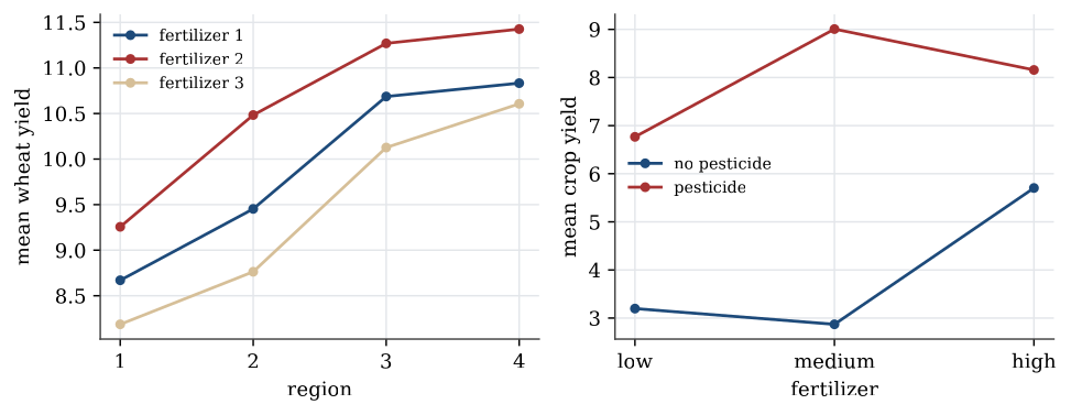
Example 3 (Pesticide and fertilizer) A crop was grown with pesticide (no or yes) and fertilizer (low, medium or high), three plots per combination. The mean yields were
| Low | Medium | High | |
|---|---|---|---|
| No pesticide | 3.20 | 2.87 | 5.70 |
| Pesticide | 6.77 | 9.01 | 8.16 |
Question. What does a two-factor analysis show?
Solution. A two-sample t test of pesticide alone, ignoring fertilizer, gives t=-7.30 and p=1.8\times10^{-6}. The two-factor analysis with interaction shows why that single number is incomplete. The interaction is enormous, F=574 on (2,12) degrees of freedom: without pesticide the yield is best at high fertilizer, with pesticide it is best at medium. The effect of pesticide is 3.57 at low fertilizer, 6.14 at medium and 2.45 at high. Reporting one average “pesticide effect” would hide that the best fertilizer level depends on whether pesticide is used. With interaction this strong, the useful summary is the table of cell means.
Randomisation and blocking
In a designed experiment, treatments are assigned to experimental units at random, so that the treatment groups are alike in every other respect. When the units fall into groups that are known to differ, such as plots in different fields, patients in different hospitals, or measurements on different days, randomising within each group, a block, removes that variation from the comparison. That is the randomised block design, analysed with block as a second factor; the tips-and-coupons example in Analysis of variance shows how much a block can matter.
Put the response in one column and each factor in another. Fit the model with lm, read the F tests in anova, check the residuals, and test the interaction before reading the main effects. A significant F says some means differ; a multiple-comparison method says which.
Questions on this topic
Open a question to attempt it. Its worked answer is folded away at the bottom of the page.
| Question | Answer |
|---|---|
| Haemoglobin and sickle-cell type | ✓ |
| Five treatments, ten pairs | ✓ |
What links here
Pages (2)
- Analysis of variance — via Bonferroni, Analysis of variance examples
- Linear model examples — via interaction
Questions and answers (1)
See also
- Articles from this chapter: Bonferroni correction · Interaction
- All data analysis chapters
- Glossary and index
- Distribution sheet and formula lookup