One-way analysis of variance
Definition taught in Analysis of variance, part of Statistical inference
One-way analysis of variance
| Type | Definition |
| Taught in | Analysis of variance |
| Part | Statistical inference |
| Properties | 2 |
| Worked examples | 4 |
| Questions using it | 4 |
In a completely randomised one-factor design, responses at level j=1,\ldots,k follow
Y_{ij}=\mu_j+\varepsilon_{ij}, \qquad \varepsilon_{ij}\ \text{independent}\ \operatorname{N}(0,\sigma^2),
with n_j observations at level j and n=\sum_j n_j. The levels are the treatments. The hypothesis of equal means is H_0:\mu_1=\cdots=\mu_k.
Properties
ANOVA sum of squares decomposition
Main article: ANOVA sum of squares decomposition
With
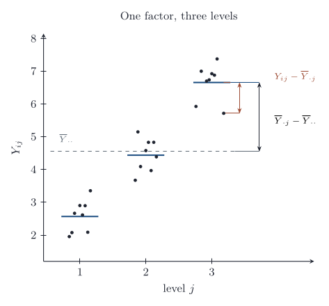
\mathrm{SS}_{\mathrm{total}}=\sum_{j=1}^k\sum_{i=1}^{n_j}(Y_{ij}-\overline Y_{\cdot\cdot})^2, \qquad \mathrm{SS}_{\mathrm{treatment}}=\sum_{j=1}^k n_j(\overline Y_{\cdot j}-\overline Y_{\cdot\cdot})^2, \qquad \mathrm{SS}_{\mathrm{error}}=\sum_{j=1}^k\sum_{i=1}^{n_j}(Y_{ij}-\overline Y_{\cdot j})^2,
the total sum of squares splits as \mathrm{SS}_{\mathrm{total}}=\mathrm{SS}_{\mathrm{treatment}}+\mathrm{SS}_{\mathrm{error}}.
ANOVA F distribution
Main article: ANOVA F distribution
In the one-way model, \mathrm{SS}_{\mathrm{error}}/\sigma^2 is \chi^2_{n-k}, and it is independent of \mathrm{SS}_{\mathrm{treatment}}. Under H_0:\mu_1=\cdots=\mu_k, \mathrm{SS}_{\mathrm{treatment}}/\sigma^2 is \chi^2_{k-1}, and therefore
F=\frac{\mathrm{SS}_{\mathrm{treatment}}/(k-1)}{\mathrm{SS}_{\mathrm{error}}/(n-k)}=\frac{\mathrm{MS}_{\mathrm{treatment}}}{\mathrm{MS}_{\mathrm{error}}}
has the F_{k-1,\,n-k} distribution.
Examples
Five varieties of corn
Worked example from Analysis of variance
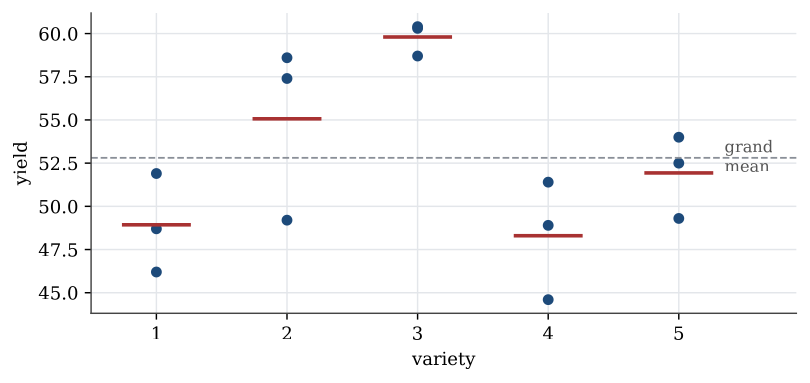
Five varieties of corn are each grown on three plots.
| Variety | 1 | 2 | 3 | 4 | 5 |
|---|---|---|---|---|---|
| Yields | 46.2, 51.9, 48.7 | 49.2, 58.6, 57.4 | 60.3, 58.7, 60.4 | 48.9, 51.4, 44.6 | 52.5, 54.0, 49.3 |
| Mean | 48.93 | 55.07 | 59.80 | 48.30 | 51.93 |
Question. Do the varieties differ in mean yield?
Solution. The grand mean is 52.81. Then \mathrm{SS}_{\mathrm{treatment}}=3\sum_j(\overline y_{\cdot j}-52.81)^2=270.3 on 4 degrees of freedom, and \mathrm{SS}_{\mathrm{error}}=105.7 on 10.
| Source | Df | SS | MS | F | p |
|---|---|---|---|---|---|
| Variety | 4 | 270.3 | 67.57 | 6.39 | 0.008 |
| Error | 10 | 105.7 | 10.57 | ||
| Total | 14 | 375.9 |
The p-value is 0.008, so the varieties differ. The pooled standard deviation is \sqrt{10.57}=3.25. The F test says only that the five means are not all equal; which varieties differ is the next question.
Five treatments for cold sores
Worked example from Analysis of variance examples
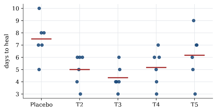
Thirty patients with cold sores were assigned at random to five treatments, six to each; treatment 1 is a placebo. The days until the sore healed were
| Placebo | T2 | T3 | T4 | T5 |
|---|---|---|---|---|
| 5 | 4 | 6 | 7 | 9 |
| 8 | 6 | 4 | 4 | 3 |
| 7 | 6 | 4 | 6 | 5 |
| 7 | 3 | 5 | 6 | 7 |
| 10 | 5 | 4 | 3 | 7 |
| 8 | 6 | 3 | 5 | 6 |
Question. Do the treatments differ in mean healing time?
Solution. The table is not in standard form: for an analysis the healing times must be one column and the treatment a factor in another. stack does that.
x <- data.frame(Placebo = c(5, 8, 7, 7, 10, 8), T2 = c(4, 6, 6, 3, 5, 6),
                T3 = c(6, 4, 4, 5, 4, 3), T4 = c(7, 4, 6, 6, 3, 5),
                T5 = c(9, 3, 5, 7, 7, 6))
coldsore <- stack(x)
names(coldsore) <- c("times", "treatment")
tapply(coldsore$times, coldsore$treatment, mean)
# Placebo  T2    T3    T4    T5
#   7.500 5.000 4.333 5.167 6.167
coldsore.lm <- lm(times ~ treatment, data = coldsore)
anova(coldsore.lm)
#           Df Sum Sq Mean Sq F value  Pr(>F)
# treatment  4 36.467  9.1167  3.896 0.01359
# Residuals 25 58.500  2.3400
Under equal means F=3.90 would come from an F_{4,25} distribution, and the p-value is 0.014, so the treatments do differ. The placebo has the longest mean healing time, 7.5 days. The residual mean square, 2.34, estimates the common variance, so the within-group standard deviation is about 1.5 days.
Heart rates in four age groups
Question page: Heart rates in four age groups
Four age groups each have 10 measurements of the increase in heart rate. The group totals are 309, 275, 295 and 282. The error sum of squares about the four group means is 935.500.
Compute the treatment sum of squares and the F statistic for equal means.
The 0.95 quantile of F_{3,36} is about 2.87. What does the test conclude at level 0.05?
The grand total is 309+275+295+282=1161, so the grand mean is 1161/40=29.025. The group means are 30.9, 27.5, 29.5 and 28.2. With 10 observations in each group,
\mathrm{SS}_{\mathrm{treatment}}=10\bigl[(30.9-29.025)^2+(27.5-29.025)^2+(29.5-29.025)^2+(28.2-29.025)^2\bigr]=67.475.
F=\frac{67.475/3}{935.500/36}=\frac{22.492}{25.986}\approx 0.866.
This is smaller than 2.87, so the test does not reject equal mean increases at level 0.05. The p-value is 0.47.
Two groups
Question page: Two groups
Show that in a one-way analysis of variance with k=2 groups, F=T^2, where T is the pooled two-sample t statistic for H_0:\mu_1=\mu_2.
With two groups, the grand mean is \overline Y_{\cdot\cdot}=(n_1\overline Y_1+n_2\overline Y_2)/n, so \overline Y_1-\overline Y_{\cdot\cdot}=n_2(\overline Y_1-\overline Y_2)/n and \overline Y_2-\overline Y_{\cdot\cdot}=-n_1(\overline Y_1-\overline Y_2)/n. Then
\mathrm{SS}_{\mathrm{treatment}}=\frac{n_1n_2^2+n_2n_1^2}{n^2}(\overline Y_1-\overline Y_2)^2=\frac{n_1n_2}{n}(\overline Y_1-\overline Y_2)^2=\frac{(\overline Y_1-\overline Y_2)^2}{1/n_1+1/n_2},
on 1 degree of freedom. The error mean square is \mathrm{SS}_{\mathrm{error}}/(n-2)=s_p^2, the pooled variance. So
F=\frac{(\overline Y_1-\overline Y_2)^2}{s_p^2(1/n_1+1/n_2)}=T^2.
Figures
Used in
- Taught in Analysis of variance, where the derivation and examples are.
- Also used in Using R · Analysis of variance examples · Linear model examples · Paired comparisons, and how far a fit is from the data
- Questions that use it (4) — Two groups · Haemoglobin and sickle-cell type · Five treatments, ten pairs · Wages, class, and gender
- All 6 questions on Analysis of variance
See also
ANOVA sum of squares decomposition · ANOVA F distribution · Contrast · Tukey intervals · Randomised block design