Random experiments and probability
Part of Probability · 17 questions on this topic · What links here
Random experiments and probability
| Part | Probability |
| Chapter | 1 of 7 in this part |
| Next | Random variables and distributions |
| Questions | 17 |
| Definitions | Sample space · Event · Probability measure · Conditional probability · Independent events |
| Results | Properties of a probability · Equally likely outcomes · Four ways of counting draws · Product rule · Law of total probability |
| Figures | 3 |
A random experiment is a procedure whose outcome is not fixed in advance, but which can still be described exactly enough that probabilities can be calculated. Tossing a coin, recording a lifetime, or drawing a sample are experiments of this kind. The model has three pieces: the set of outcomes that can occur, the events one might ask about, and a probability for each event.
The same conditional-probability identity, written for densities and read as a rule for updating a prior, is Bayes’ rule on the Bayesian foundations page. This chapter keeps the event form.
Randomness as a model
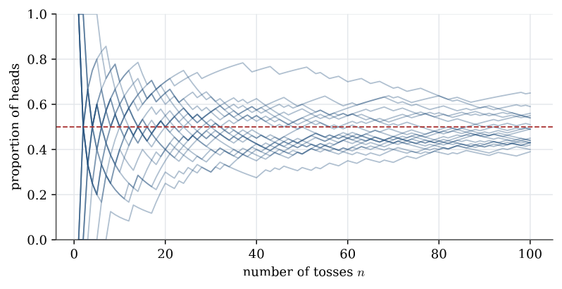
Toss a fair coin 100 times and record a 1 for heads and a 0 for tails. Nobody can say in advance what the sequence will be. Yet the proportion of heads after n tosses behaves in a predictable way: it wanders a good deal for small n and settles near 1/2 as n grows. Probability is the mathematics of experiments like this one, whose single outcomes are unpredictable but whose long-run behaviour is not.
The same shape of question turns up far from coins. A factory weighs 10 bags of sugar each hour and raises an alarm when the average crosses a control limit; where to put the limits depends on how much the hourly average varies when nothing is wrong. Engineers watch 1000 components for 50 000 hours and tabulate the fraction failed by each time; the question is which continuous lifetime distribution that table is a noisy picture of. Each of these is a random experiment, and each needs the three pieces below: the outcomes, the events, and the probabilities.
Example 1 (A four-engine aeroplane) An aeroplane has engines 1 and 2 on the left wing and 3 and 4 on the right. It can fly as long as at least one engine on each wing works. Each engine fails during a flight with probability q, independently of the others.
Question. Describe the sample space and the event that the aeroplane can fly, and find its probability.
Solution. Record which engines work: an outcome is a vector in \{0,1\}^4, so there are 2^4=16 outcomes. Let A_i be the event that engine i works. The aeroplane can fly on the event
(A_1\cup A_2)\cap(A_3\cup A_4).
A wing fails only if both its engines fail, with probability q^2, so by independence of the two wings
\mathbb{P}\{(A_1\cup A_2)\cap(A_3\cup A_4)\}=(1-q^2)^2.
With q=0.1 that is 0.9801. A single engine fails one flight in ten, but the aeroplane only about one flight in fifty. Redundancy turns unreliable parts into a reliable system, which is the subject of Reliability.
Outcomes and events
Definition 1 (Sample space) The sample space \Omega of a random experiment is the set of all outcomes that experiment can produce.
The sample space is a modelling choice, not a fact about the apparatus. Three tosses of a coin can be recorded as the sequence of faces, so \Omega=\{0,1\}^3, or only as the number of heads, so \Omega=\{0,1,2,3\}. Both descriptions are correct. They answer different questions.
A few standard spaces:
- two dice in order, \Omega=\{1,\ldots,6\}^2;
- a lifetime in days, \Omega=[0,\infty);
- the number of calls in a fixed interval, \Omega=\{0,1,2,\ldots\};
- the heights of ten people, \Omega=\mathbb{R}^{10}.
A space is discrete when its outcomes can be listed, finite or countably infinite. It is continuous when they cannot, as with an interval of real numbers.
Definition 2 (Event) An event is a subset of the sample space. The event occurs when the outcome lies in that subset.
If A and B are events, then A\cup B occurs when at least one of them does, A\cap B occurs when both do, and the complement A^c occurs when A does not. The empty set is the impossible event and \Omega is the certain event. A\subset B means that A cannot occur unless B does.
For any collection of events, De Morgan’s laws swap unions and intersections under complements:
\Bigl(\bigcup_i A_i\Bigr)^c=\bigcap_i A_i^c, \qquad \Bigl(\bigcap_i A_i\Bigr)^c=\bigcup_i A_i^c.
Read the first one as a reliability statement. If A_i means that component i works, the left-hand side is “the parallel system of those components has failed”, and the right-hand side is “every component has failed”.
Systems of three components show how events are built from simpler ones. Let A_i be the event that component i works. A series system works only if every component works, the event A_1\cap A_2\cap A_3. A parallel system works if at least one does, A_1\cup A_2\cup A_3. A 2-out-of-3 system works if at least two do,
(A_1\cap A_2)\cup(A_1\cap A_3)\cup(A_2\cap A_3).
By De Morgan’s laws, the series system fails on A_1^c\cup A_2^c\cup A_3^c, when any component fails, and the parallel system fails on A_1^c\cap A_2^c\cap A_3^c, when all of them do.
Probability
Definition 3 (Probability measure) A probability \mathbb{P} assigns a number to each event and satisfies three axioms: \mathbb{P}(A)\ge 0, \mathbb{P}(\Omega)=1, and for any sequence of disjoint events,
\mathbb{P}\Bigl(\bigcup_i A_i\Bigr)=\sum_i \mathbb{P}(A_i).
The third axiom is the sum rule. If an event can happen in mutually exclusive ways, its probability is the sum of those ways. Area on a page works the same way: the area of a union of non-overlapping regions is the sum of the areas. Probability is that kind of measure, with total measure one.
Theorem 1 (Properties of a probability) For events A and B,
- \mathbb{P}(\emptyset)=0.
- A\subset B implies \mathbb{P}(A)\le \mathbb{P}(B).
- \mathbb{P}(A)\le 1.
- \mathbb{P}(A^c)=1-\mathbb{P}(A).
- \mathbb{P}(A\cup B)=\mathbb{P}(A)+\mathbb{P}(B)-\mathbb{P}(A\cap B).
The empty set is disjoint from \Omega, so the sum rule gives \mathbb{P}(\Omega)=\mathbb{P}(\Omega)+\mathbb{P}(\emptyset). The complement formula is the sum rule on the disjoint union \Omega=A\cup A^c. For the union formula, write A\cup B as the disjoint union of A and B\cap A^c, and write B as the disjoint union of A\cap B and B\cap A^c. Subtracting the two expansions cancels \mathbb{P}(B\cap A^c).
On a discrete space \Omega=\{a_1,a_2,\ldots\} it is enough to give a weight p_i=\mathbb{P}(\{a_i\}) to each outcome, with p_i\ge 0 and \sum_i p_i=1. An event then has probability equal to the total weight of the outcomes it contains. On a continuous space this fails: each single point must have probability zero, or an uncountable sum of equal positive weights could not be one. Probabilities are assigned to intervals, or to other sets with a length or a volume.
Theorem 2 (Equally likely outcomes) If \Omega is finite and every outcome has the same probability, then for every event A
\mathbb{P}(A)=\frac{|A|}{|\Omega|}.
A fair die is the model case: \Omega=\{1,\ldots,6\} and \mathbb{P}(A)=|A|/6. Drawing a point “at random” from [0,1] is the continuous analogue. The sample space is the interval, and
\mathbb{P}([a,b])=b-a, \qquad 0\le a\le b\le 1.
The probability of a set is its length. A single point has length zero, so it has probability zero, even though it is a possible outcome.
Counting
When outcomes are equally likely, a probability is a ratio of two counts. Many counts are one of four urn problems. An urn holds n distinct balls, and k of them are drawn. The draw may or may not record order, and it may or may not replace each ball.
Proposition 1 (Four ways of counting draws)
| Order recorded | Replacement | Number of outcomes |
|---|---|---|
| yes | yes | n^k |
| yes | no | n!/(n-k)! |
| no | no | \binom{n}{k} |
| no | yes | \binom{n+k-1}{k} |
Ordered outcomes are written as vectors, so (1,2,3)\ne(3,2,1). Unordered outcomes are written as sets, so \{1,2,3\}=\{3,2,1\}.
The first row fills k positions, each with n choices. The second row is the same except that a ball already drawn is no longer available: n(n-1)\cdots(n-k+1). The third row forgets the order, and each unordered set of size k corresponds to k! ordered draws, so the count is divided by k!. That quotient is the binomial coefficient
\binom{n}{k}=\frac{n!}{k!\,(n-k)!}.
The fourth row, unordered draws with replacement, counts the multisets of size k from n labels. It is less common in the calculations below; the first three rows cover sequences, permutations and combinations.
A multiple-choice paper with 20 questions and 3 answers each is the first row: 3^{20} scripts. The number of ways to award first, second and third place among 8 horses is the second row: 8\times 7\times 6. The number of ways to choose 3 discs from 20, order irrelevant, is \binom{20}{3}.
Two counting facts are used often enough to keep them separate. The number of ways to arrange n distinct objects is n!. If a word has repeated letters, divide by the factorial of each repetition: “arrange” has 7 letters with “a” and “r” doubled, so it has 7!/(2!\,2!) distinct rearrangements.
Example 2 (The birthday problem) A group has n people. Ignore leap days and assume each birthday is equally likely to be any of 365 days, independently.
Question. What is the probability that at least two people share a birthday?
Solution. The birthday count is the second row of the table against the first. The probability that all birthdays differ is
\frac{365\times 364\times\cdots\times(365-n+1)}{365^n},
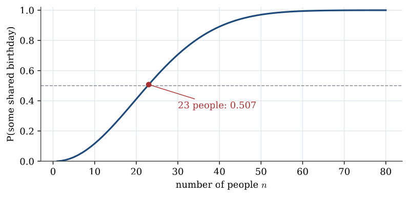
provided n\le 365, and zero otherwise. The numerator is the number of injective assignments of days, and the denominator is the number of assignments with replacement. The probability of a shared birthday is one minus this. It passes one half at n=23, where it is 0.507, and reaches 0.891 at n=40 and 0.970 at n=50.
The surprise comes from counting the wrong thing. 23 people seem few against 365 days, but they form \binom{23}{2}=253 pairs, and any one of those pairs can match.
Conditional probability
Definition 4 (Conditional probability) If \mathbb{P}(B)>0, the conditional probability of A given B is
\mathbb{P}(A\mid B)=\frac{\mathbb{P}(A\cap B)}{\mathbb{P}(B)}.
Conditioning on B replaces the sample space by B and renormalises. In the equally likely case this is just the count of outcomes in A\cap B divided by the count of outcomes in B.
Two dice are thrown and the sum is 10, so B=\{(4,6),(5,5),(6,4)\}. Exactly one six has been thrown on the event A\cap B=\{(4,6),(6,4)\}. Every ordered pair is equally likely, so \mathbb{P}(A\mid B)=2/3.
Example 3 (The Monty Hall problem) A prize is equally likely behind curtain A, B or C. The contestant picks A. The host, who knows where the prize is, always opens a different curtain that has no prize, choosing at random when both remaining curtains are empty.
Question. Suppose the host opens B. Should the contestant switch to C?
Solution. The definition of conditional probability settles it without any story about psychology. The four atoms that can occur, with their probabilities, are: prize behind A and host opens B (1/6), prize behind A and host opens C (1/6), prize behind B and host opens C (1/3), prize behind C and host opens B (1/3). The observed event is the two atoms in which B is opened, with total probability 1/6+1/3=1/2. The prize is behind A in only the first of those atoms, so
\mathbb{P}(\text{prize behind }A\mid \text{host opens }B)=\frac{1/6}{1/2}=\frac13,
and the probability it is behind C is 2/3. Switching wins with probability 2/3.
The tempting answer, one half each, forgets that the host’s choice depends on where the prize is. When the contestant’s first pick is wrong, which happens two times in three, the host is forced to reveal the only other empty curtain.
Theorem 3 (Product rule) If \mathbb{P}(A_1\cap\cdots\cap A_{n-1})>0, then
\mathbb{P}(A_1\cap\cdots\cap A_n) =\mathbb{P}(A_1)\,\mathbb{P}(A_2\mid A_1)\,\mathbb{P}(A_3\mid A_1\cap A_2)\cdots\mathbb{P}(A_n\mid A_1\cap\cdots\cap A_{n-1}).
Each factor is the definition of conditional probability, and the intermediate intersections cancel.
Three black balls drawn without replacement from an urn with 5 black and 5 white balls have probability
\frac{5}{10}\times\frac{4}{9}\times\frac{3}{8}=\frac{1}{12}.
The birthday probability above is the same rule. Let A_k be the event that the first k birthdays are all different. Then A_n=A_1\cap\cdots\cap A_n and \mathbb{P}(A_k\mid A_{k-1})=(365-k+1)/365.
Theorem 4 (Law of total probability) If B_1,\ldots,B_n are disjoint and their union is \Omega, then for every event A
\mathbb{P}(A)=\sum_{i=1}^n \mathbb{P}(A\mid B_i)\,\mathbb{P}(B_i).
The events A\cap B_i are disjoint and exhaust A, so the sum rule applies, and each term is the product rule.
Dividing one term by the sum is Bayes’ rule for events. For each j,
\mathbb{P}(B_j\mid A)=\frac{\mathbb{P}(A\mid B_j)\,\mathbb{P}(B_j)}{\sum_{i=1}^n \mathbb{P}(A\mid B_i)\,\mathbb{P}(B_i)},
provided the denominator is positive. This is the same algebra as the density form on Bayesian foundations. The difference is the object that carries the probability. Here it is an event. There it is an unknown parameter, and the factors are a likelihood and a prior.
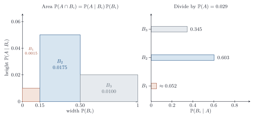
Example 4 (Three factories) A chip is made in factory 1, 2 or 3 with probabilities 0.15, 0.35 and 0.50, and the defective rates are 0.01, 0.05 and 0.02.
Question. A chip in hand is defective. What is the probability that it came from factory 1?
Solution. By Bayes’ rule, the probability it came from factory 1 is
\frac{0.15\times 0.01}{0.15\times 0.01+0.35\times 0.05+0.50\times 0.02}=\frac{0.0015}{0.029}\approx 0.052.
The rare factory is unlikely to be the source, because the two larger factories produce more defectives in total even though each chip from factory 1 is less often defective.
The same calculation gives 0.0175/0.029=0.603 for factory 2 and 0.010/0.029=0.345 for factory 3. The denominator, 0.029, is the overall defective rate, from the law of total probability.
Independence
Definition 5 (Independent events) Events A_1,A_2,\ldots are mutually independent when, for every finite subcollection,
\mathbb{P}(A_{i_1}\cap\cdots\cap A_{i_k})=\mathbb{P}(A_{i_1})\cdots\mathbb{P}(A_{i_k}).
For two events with positive probability this is the same as \mathbb{P}(A\mid B)=\mathbb{P}(A): learning that B occurred does not change the probability of A. The product form is the one to use in calculations, and it still makes sense if one of the events is empty. Pairwise products are not enough for three or more events. Mutual independence asks for every subcollection.
Independence is usually an assumption of the model, not a theorem about the apparatus. It says which probability measure is being used.
A coin with heads-probability p is tossed n times, and the tosses are independent. The sample space is \{0,1\}^n. Any particular sequence with k heads and n-k tails has probability p^k(1-p)^{n-k}. There are \binom{n}{k} such sequences, so the probability of exactly k heads is
\binom{n}{k}p^k(1-p)^{n-k}, \qquad k=0,1,\ldots,n.
That is the binomial distribution. Its mean, variance and the rest of the named distributions are on the common distributions page. Tossing until the first head, with the same independence, gives the geometric distribution on \{1,2,\ldots\}: the first head arrives at toss k with probability (1-p)^{k-1}p.
Specify the outcomes, the events, and the probability. Equally likely finite spaces reduce the probability to a count. Conditioning replaces the space by the event that was observed. Independence is the assumption that lets a joint probability factor into a product.
Questions on this topic
Open a question to attempt it. Its worked answer is folded away at the bottom of the page.
What links here
Pages (4)
- Random variables and distributions — via sample space, Random experiments and probability
- Joint distributions — via Conditional probability, Random experiments and probability, product rule, law of total probability
- Statistical inference — via Random experiments and probability
- Studies, data, and evidence — via Random experiments and probability
Questions and answers (8)
- Three coin tosses · Weights on the two coin spaces · Three cards in order · One of each court card (answer) · Information about one die (answer) · A channel with unequal inputs (answer) · The sum of two dice · A point in a triangle (answer)
See also
- Articles from this chapter: Sample space · Event · Probability measure · Properties of a probability · Equally likely outcomes · Four ways of counting draws · Conditional probability · Product rule · Law of total probability · Independent events
- All probability chapters
- Glossary and index
- Distribution sheet and formula lookup