Geometric distribution
Definition taught in Random variables and distributions, part of Probability · Also on the distribution sheet
Geometric distribution
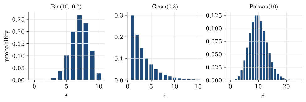
| Notation | x\sim\operatorname{Geom}(p) |
| Parameters | p\in(0,1] |
| Support | x=1,2,3,\ldots |
| Mass function | p(x)=p(1-p)^{x-1} |
| Mean | \mathbb{E}(x)=1/p |
| Variance | \operatorname{Var}(x)=(1-p)/p^{2} |
| Taught in | Random variables and distributions |
| Part | Probability |
| Properties | 1 |
| Worked examples | 4 |
| Questions using it | 1 |
From the distribution sheet.
X has the geometric distribution with success probability p\in(0,1], written X\sim\operatorname{Geom}(p), when
\mathbb{P}(X=x)=(1-p)^{x-1}p,\qquad x=1,2,\ldots
It is the trial on which the first success occurs, in a sequence of independent \operatorname{Bern}(p) trials. Then \mathbb{E} X=1/p and \operatorname{Var}(X)=(1-p)/p^2.
Properties
Memoryless property
Main article: Memoryless property
A positive random variable X is memoryless when \mathbb{P}(X>s+t\mid X>s)=\mathbb{P}(X>t) for all s,t>0. The exponential distributions are the continuous memoryless laws, and the geometric distributions are the discrete ones.
For the exponential law with rate \lambda, the survival probability is e^{-\lambda x}, so
\mathbb{P}(X>s+t\mid X>s)=\frac{e^{-\lambda(s+t)}}{e^{-\lambda s}}=e^{-\lambda t}.
The geometric calculation is the same with (1-p)^{s+t} in place of e^{-\lambda(s+t)}.
Examples
Question 11. Geometric success probability
Question page: Question 11. Geometric success probability
Let x_1,\ldots,x_n be iid with
f(x\mid p)=(1-p)^{x}p, \quad x=0,1,2,\ldots,
and p\sim\operatorname{Beta}(\alpha,\beta).
(i) Find the posterior distribution of p and identify it. [3 marks]
(ii) Is this prior conjugate? [1 mark]
(iii) Show that a \operatorname{Beta}(a,b) mean equals a/(a+b). [2 marks]
(iv) Hence show that \mathbb{E}(p\mid{\boldsymbol{x}})=(\alpha+n)/(\alpha+\beta+n+n\bar x). [1 mark]
(v) What happens to the posterior mean as n\to\infty? [1 mark]
(vi) What happens if \alpha,\beta\to 0? [1 mark]
(vii) Complete: “The effect of the prior hyperparameters \alpha,\beta on the posterior mean of p is like…” [2 marks]
Definitions. Here X_i counts failures before the first success, so its support begins at zero. Each observation represents one success and x_i failures. Put F=\sum_i x_i=n\bar x. The beta density is p^{\alpha-1}(1-p)^{\beta-1}/B(\alpha,\beta) on 0<p<1. This geometric convention differs from the trial-count convention in Question 6 by one.
(i) The likelihood is p^{n}(1-p)^{\sum x_i}. The beta prior contributes p^{\alpha-1}(1-p)^{\beta-1}, so
\boxed{p\mid{\boldsymbol{x}}\sim\operatorname{Beta}\bigl(\alpha+n,\;\beta+\textstyle\sum_{i=1}^{n}x_i\bigr).}
(ii) Yes. The posterior is beta, the same family as the prior.
(iii) For a>0 and b>0, the expectation integral is
\mathbb{E}(P)=\frac1{B(a,b)}\int_0^1 p^a(1-p)^{b-1}\,dp =\frac{B(a+1,b)}{B(a,b)}.
Using B(a,b)=\Gamma(a)\Gamma(b)/\Gamma(a+b) and \Gamma(a+1)=a\Gamma(a),
\frac{B(a+1,b)}{B(a,b)} = \frac{\Gamma(a+1)\Gamma(a+b)}{\Gamma(a)\Gamma(a+b+1)} = \frac{a}{a+b},
and this ratio is the beta mean.
(iv) By (i) and (iii),
\mathbb{E}(p\mid{\boldsymbol{x}}) = \frac{\alpha+n}{\alpha+\beta+n+n\bar x}.
(v) Divide the numerator and denominator by n:
\mathbb{E}(p\mid{\boldsymbol{x}})=\frac{1+\alpha/n}{1+\bar x+(\alpha+\beta)/n}.
For fixed prior parameters this approaches the data-based estimate 1/(1+\bar x). The log-likelihood is n\log p+F\log(1-p), and setting its derivative to zero gives \hat p=n/(n+F) when F>0. If the data come from the model at p_0, then \bar X_n\to(1-p_0)/p_0 and both estimates converge to p_0.
(vi) If \alpha,\beta\to 0, the posterior mean tends to n/(n+n\bar x)=1/(1+\bar x). The prior drops out.
This is a limit of proper beta priors, not substitution of \alpha=\beta=0 into a proper prior density. If F=0, the limiting estimate is the boundary value 1 and the limiting beta kernel is not a proper density; the posteriors for positive hyperparameters remain proper.
(vii) The effect is like \alpha prior successes and \beta prior failures, added to the n observed successes and \sum x_i observed failures.
An exact weighted-average expression makes that interpretation explicit:
\mathbb{E}(p\mid{\boldsymbol{x}}) =\frac{\alpha+\beta}{\alpha+\beta+n+F}\frac{\alpha}{\alpha+\beta} +\frac{n+F}{\alpha+\beta+n+F}\frac{n}{n+F}.
The beta prior mean and the observed success fraction are weighted by their respective total counts. These pseudo-counts describe the posterior-mean update; the powers in the prior density itself are \alpha-1 and \beta-1.
A geometric observation and a uniform prior
Question page: A geometric observation and a uniform prior
Let X be the number of coin tosses up to and including the first head. Thus
\mathbb{P}(X=x\mid\theta)=\theta(1-\theta)^{x-1}, \qquad x=1,2,\ldots,
where \theta is the probability of a head. Use the prior \theta\sim\operatorname{Unif}(0,1).
Find and identify p(\theta\mid x).
Discuss whether the prior was intended to be informative and whether it is conjugate.
Find the posterior mode.
Find \mathbb{E}(\theta\mid x).
Express the posterior mean as a convex combination of the prior mean and the maximum-likelihood estimate of \theta.
Give an equivalent-prior-observations interpretation, and state which pseudo-count convention you are using.
Question. Let X be the number of coin tosses up to and including the first head. Thus
\mathbb{P}(X=x\mid\theta)=\theta(1-\theta)^{x-1}, \qquad x=1,2,\ldots,
where \theta is the probability of a head. Use the prior \theta\sim\operatorname{Unif}(0,1).
Find and identify p(\theta\mid x).
Discuss whether the prior was intended to be informative and whether it is conjugate.
Find the posterior mode.
Find \mathbb{E}(\theta\mid x).
Express the posterior mean as a convex combination of the prior mean and the maximum-likelihood estimate of \theta.
Give an equivalent-prior-observations interpretation, and state which pseudo-count convention you are using.
Solution.
- The prior density is one on (0,1), so Bayes’ rule gives \begin{align*} p(\theta\mid x) &\propto \mathbb{P}(X=x\mid\theta)p(\theta)\\ &=\theta(1-\theta)^{x-1}\\ &=\theta^{2-1}(1-\theta)^{x-1}. \end{align*} The normalising integral is
\int_0^1\theta(1-\theta)^{x-1}\,\mathrm{d}\theta =B(2,x) =\frac{\Gamma(2)\Gamma(x)}{\Gamma(x+2)} =\frac{1}{x(x+1)}.
Consequently
p(\theta\mid x)=x(x+1)\theta(1-\theta)^{x-1}, \qquad \boxed{\theta\mid x\sim\operatorname{Beta}(2,x)}.
The uniform prior was chosen to give equal density to equal-length intervals of \theta, so it was intended as a non-informative prior on this particular scale. That description is not invariant under a transformation of \theta. Since \operatorname{Unif}(0,1)=\operatorname{Beta}(1,1) and the Beta family is conjugate to this geometric likelihood, the prior is conjugate.
A \operatorname{Beta}(a,b) density has interior mode (a-1)/(a+b-2) when a,b>1. Here this gives
\operatorname{mode}(\theta\mid x) =\frac{2-1}{2+x-2}=\boxed{\frac1x}.
For x=1 this is the boundary mode at one.
- The posterior mean is
\boxed{\mathbb{E}(\theta\mid x)=\frac{2}{x+2}}.
The prior mean is 1/2. To obtain the maximum-likelihood estimator, differentiate the log likelihood: \begin{align*} \ell(\theta)&=\log\theta+(x-1)\log(1-\theta),\\ \ell'(\theta)&=\frac1\theta-\frac{x-1}{1-\theta}. \end{align*} Setting \ell'(\theta)=0 gives 1-\theta=(x-1)\theta, hence \widehat\theta_{\mathrm{MLE}}=1/x. With w=2/(x+2), \begin{align*} w\mathbb{E}(\theta)+(1-w)\widehat\theta_{\mathrm{MLE}} &=\frac{2}{x+2}\frac12 +\left(1-\frac{2}{x+2}\right)\frac1x\\ &=\frac1{x+2}+\frac{x}{x+2}\frac1x\\ &=\frac2{x+2}\\ &=\mathbb{E}(\theta\mid x). \end{align*}
Under the posterior-mean concentration convention, \operatorname{Beta}(1,1) has total prior weight two with one prior head and one prior tail: it behaves like one head among two prior tosses. Under the kernel exponent convention, however, the prior contributes \alpha-1=0 powers of \theta and \beta-1=0 powers of 1-\theta. These are two different pseudo-count conventions; the first is the one used in the requested linear combination.
Waiting for double six
Question page: Waiting for double six
Two fair dice are thrown repeatedly until their sum is 12.
Find the probability that this takes exactly 10 throws.
Find the probability that it takes at most 100 throws.
A throw shows double six with probability 1/36. The number of throws required is geometric, starting at 1.
(35/36)^9(1/36)\approx 0.0216.
The probability that the first 100 throws all fail is (35/36)^{100}, so the probability of success by throw 100 is 1-(35/36)^{100}\approx 0.940.
Expected wait for double six
Question page: Expected wait for double six
Two fair dice are thrown until both faces are six. Find the expected number of throws.
The number of throws is geometric, starting at 1, with success probability 1/36. The expectation is 36.
Used in
- Taught in Random variables and distributions, where the derivation and examples are.
- Also used in Random experiments and probability
- Questions that use it (1) — A walk with a floor (answer)
- All 27 questions on Random variables and distributions
See also
Memoryless property · Random variable · Cumulative distribution function · Discrete distribution · Continuous distribution · Expectation · Expectation of a function · Variance