Beta distribution
Definition taught in The Beta–Binomial model, part of Bayesian statistics · Also on the distribution sheet
Beta distribution
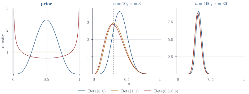
| Notation | x\sim\operatorname{Beta}(\alpha,\beta) |
| Parameters | \alpha,\beta>0 |
| Support | 0<x<1 |
| Density | p(x)=\frac{\Gamma(\alpha+\beta)}{\Gamma(\alpha)\Gamma(\beta)}x^{\alpha-1}(1-x)^{\beta-1} |
| Mean | \mathbb{E}(x)=\alpha/(\alpha+\beta) |
| Mode | (\alpha-1)/(\alpha+\beta-2) for \alpha,\beta>1 |
| Variance | \operatorname{Var}(x)=\alpha\beta/((\alpha+\beta)^{2}(\alpha+\beta+1)) |
| Conjugate prior for | X\mid p\sim\operatorname{Bin}(n,p), giving p\mid x\sim\operatorname{Beta}(\alpha+x,\beta+n-x) |
| Taught in | The Beta–Binomial model |
| Part | Bayesian statistics |
| Properties | 4 |
| Worked examples | 2 |
| Questions using it | 5 |
From the distribution sheet; mode and conjugate pairs from the formula lookup.
For \alpha,\beta>0, the Beta density is p(\theta\mid\alpha,\beta) =\frac{1}{B(\alpha,\beta)} \theta^{\alpha-1}(1-\theta)^{\beta-1}, \qquad 0<\theta<1, where
B(\alpha,\beta) =\int_0^1t^{\alpha-1}(1-t)^{\beta-1}\,\mathrm{d} t =\frac{\Gamma(\alpha)\Gamma(\beta)} {\Gamma(\alpha+\beta)}.
Properties
Beta–Binomial conjugacy
Main article: Beta–Binomial conjugacy
\boxed{ \theta\mid x\sim \operatorname{Beta}(\alpha+x,\beta+n-x)}.
The Beta distribution is the two-category Dirichlet
Main article: The Beta distribution is the two-category Dirichlet
When K=2, write p_1=p and p_2=1-p. Restricting the Dirichlet density to the one-dimensional simplex gives
p(p\mid\alpha_1,\alpha_2) =\frac{\Gamma(\alpha_1+\alpha_2)} {\Gamma(\alpha_1)\Gamma(\alpha_2)} p^{\alpha_1-1}(1-p)^{\alpha_2-1},
which is exactly \operatorname{Beta}(\alpha_1,\alpha_2). The Dirichlet is therefore a genuine extension of the Beta family rather than merely a similar-looking density.
Beta–Binomial posterior prediction
Main article: Beta–Binomial posterior prediction
If \theta\mid x\sim\operatorname{Beta}(a,b) and, conditionally on \theta, \widetilde X\sim\operatorname{Bin}(m,\theta), then
\mathbb{P}(\widetilde X=k\mid x) =\binom mk\frac{B(k+a,m-k+b)}{B(a,b)}, \qquad k=0,\ldots,m.
For one future Bernoulli observation, \mathbb{P}(\widetilde Y=1\mid x)=a/(a+b).
Two pseudo-count conventions
Main article: Two pseudo-count conventions
For posterior means, (\alpha,\beta) act as prior success and failure counts. For an interior posterior mode, the corresponding counts are (\alpha-1,\beta-1). A pseudo-count statement is incomplete unless the posterior summary being interpreted is also named.
Examples
Q6. Beta-Binomial conjugacy and prior influence
Question page: Q6. Beta-Binomial conjugacy and prior influence
Suppose X\mid\theta\sim\operatorname{Bin}(n,\theta), \qquad \theta\sim\operatorname{Beta}(a,b), where n\geq1, a,b>0, and the observed value of X is x.
(a) Derive the posterior density of \theta. Identify its distribution, parameters, and support. [3 marks]
(b) Express the posterior mean as a weighted average of the prior mean and x/n. Explain how the weight on the prior changes as n increases, with a and b fixed. [3 marks]
(c) Another statistician instead uses a prior uniform on (0,1/2). If x/n=4/5, can the posterior assign positive probability to \theta>1/2? Explain why or why not. [2 marks]
(d) Under squared-error loss, explain why the posterior mean is the Bayes estimate. Is it necessarily the Bayes estimate under a different loss? [2 marks]
Definitions. For a,b>0, a \operatorname{Beta}(a,b) density is \theta^{a-1}(1-\theta)^{b-1}/B(a,b) on (0,1), where B(a,b)=\int_0^1u^{a-1}(1-u)^{b-1}\,du. Here x is a Binomial success count out of known n. A Bayes estimate is an action d minimising posterior expected loss. Part (c) substitutes a restricted prior; part (d) returns to the Beta prior from (a).
(a) Posterior distribution
The likelihood and prior kernels are p(x\mid\theta)\propto\theta^x(1-\theta)^{n-x}, \qquad p(\theta)\propto\theta^{a-1}(1-\theta)^{b-1}. Therefore, \begin{aligned} p(\theta\mid x) &\propto p(x\mid\theta)p(\theta)\\ &\propto \theta^{a+x-1}(1-\theta)^{b+n-x-1}, \qquad 0<\theta<1. \end{aligned} Thus \boxed{ \theta\mid x\sim\operatorname{Beta}(a+x,b+n-x) }. The normalised posterior density is p(\theta\mid x) =\frac{\theta^{a+x-1}(1-\theta)^{b+n-x-1}} {B(a+x,b+n-x)}, \qquad 0<\theta<1.
(b) Posterior mean and prior influence
The posterior mean is \mathbb{E}(\theta\mid x)=\frac{a+x}{a+b+n}. Since the prior mean is \mathbb{E}(\theta)=a/(a+b), \begin{aligned} \mathbb{E}(\theta\mid x) &= \frac{a+b}{a+b+n}\frac{a}{a+b} +\frac{n}{a+b+n}\frac{x}{n}\\ &= \boxed{ \frac{a+b}{a+b+n}\mathbb{E}(\theta) +\frac{n}{a+b+n}\frac{x}{n} }. \end{aligned} The two weights sum to one. With a and b fixed, the prior weight (a+b)/(a+b+n) decreases to zero as n\to\infty, while the data weight increases to one.
(c) Restricted prior support
No. A prior uniform on (0,1/2) has density zero for \theta>1/2. Because p(\theta\mid x)\propto p(x\mid\theta)p(\theta), the posterior is also zero wherever the prior is zero. Hence \boxed{\mathbb{P}(\theta>1/2\mid x)=0}, even when x/n=4/5. The likelihood can reweight values inside the prior support, but it cannot create posterior mass outside that support.
(d) Bayes estimate under squared-error loss
Write m=\mathbb{E}(\theta\mid x) and expand \theta-d=(\theta-m)+(m-d). The cross term has posterior expectation 2(m-d)\mathbb{E}(\theta-m\mid x)=0. Consequently, for an estimate d, the posterior expected squared loss is \begin{aligned} \mathbb{E}\bigl[(\theta-d)^2\mid x\bigr] &= \operatorname{Var}(\theta\mid x) +\bigl\{\mathbb{E}(\theta\mid x)-d\bigr\}^2. \end{aligned} The variance term does not depend on d, so this expression is minimised by \boxed{ \widehat{\theta}_{\mathrm{Bayes}} =\mathbb{E}(\theta\mid x) =\frac{a+x}{a+b+n}. } The Bayes estimate depends on the loss function: for example, absolute-error loss gives a posterior median rather than necessarily the posterior mean.
Q23. Rat-tumour studies and hierarchical shrinkage
Question page: Q23. Rat-tumour studies and hierarchical shrinkage
[12 marks]
Suppose J related studies record tumour counts Y_j\mid\theta_j\sim\operatorname{Binomial}(n_j,\theta_j), \qquad j=1,\ldots,J, independently conditional on the study rates. Assume \theta_j\mid\alpha,\beta \overset{\mathrm{iid}}{\sim}\operatorname{Beta}(\alpha,\beta), \qquad \alpha\sim\operatorname{Exp}(1),\quad \beta\sim\operatorname{Exp}(1), where the two hyperpriors are independent. Write \mathbf y=(y_1,\ldots,y_J); the sample sizes n_j are known. You may use B(a,b)=\int_0^1 t^{a-1}(1-t)^{b-1}\,dt, \qquad f(\theta\mid a,b)=\frac{\theta^{a-1}(1-\theta)^{b-1}}{B(a,b)}.
(a) [2 marks] Derive and identify the full conditional distribution \theta_j\mid\alpha,\beta,\mathbf y.
(b) [3 marks] For this part only, fix \alpha=2 and \beta=8. Two studies report (y_1,n_1)=(4,10),\qquad (y_2,n_2)=(40,100). Calculate both posterior means. Although both observed proportions equal 0.4, explain why the posterior means differ and identify which study experiences stronger shrinkage.
(c) [4 marks] Return to unknown \alpha,\beta. Integrate out the study rates to derive:
(i) the marginal probability \mathbb{P}(Y_j=y_j\mid\alpha,\beta);
(ii) the marginal posterior kernel p(\alpha,\beta\mid\mathbf y).
Express your answers using Beta functions. Explain why the Beta prior’s normalising factor cannot be discarded when deriving this hyperparameter posterior.
(d) [3 marks] Explain how the full Bayesian model allows studies to share information. What uncertainty is omitted if \alpha,\beta are instead estimated from the data and then treated as known?
Definitions. Study j has observed count y_j, known size n_j, and unknown rate \theta_j; \alpha,\beta>0 are shared hyperparameters. A \operatorname{Beta}(\alpha,\beta) density is \theta^{\alpha-1}(1-\theta)^{\beta-1}/B(\alpha,\beta) on (0,1), where B(a,b)=\int_0^1u^{a-1}(1-u)^{b-1}\,du. \operatorname{Exp}(1) uses rate one. Partial pooling allows different study rates linked through a common population distribution.
Assumptions. The hierarchy assumes conditional independence of studies given their rates, and iid Beta rates given \alpha,\beta. Thus its joint density factors as p(\alpha)p(\beta)\prod_jp(\theta_j\mid\alpha,\beta)p(y_j\mid\theta_j), with independent rate-one exponential hyperpriors. Only in part (b) are the hyperparameters fixed at the supplied values.
(a) Full conditional for a study rate. Holding \alpha,\beta fixed, the factors involving \theta_j are \begin{aligned} p(\theta_j\mid\alpha,\beta,\mathbf y) &\propto p(y_j\mid\theta_j)p(\theta_j\mid\alpha,\beta)\\ &\propto\theta_j^{y_j}(1-\theta_j)^{n_j-y_j} \theta_j^{\alpha-1}(1-\theta_j)^{\beta-1}\\ &=\theta_j^{\alpha+y_j-1}(1-\theta_j)^{\beta+n_j-y_j-1}. \end{aligned} Therefore \boxed{\theta_j\mid\alpha,\beta,\mathbf y \sim\operatorname{Beta}(\alpha+y_j,\beta+n_j-y_j),\qquad 0<\theta_j<1.} Conditional on the hyperparameters and data, the study rates are independent. Other studies’ observations affect this study’s marginal posterior through learning \alpha,\beta, not through an additional factor in this full conditional.
(b) Posterior means and shrinkage. For fixed \alpha=2, \beta=8, the population mean is \frac{\alpha}{\alpha+\beta}=\frac2{10}=0.2. The two posteriors are \theta_1\mid\alpha=2,\beta=8,\mathbf y\sim\operatorname{Beta}(6,14), \theta_2\mid\alpha=2,\beta=8,\mathbf y\sim\operatorname{Beta}(42,68). Thus their posterior means are \boxed{\mathbb{E}(\theta_1\mid\alpha=2,\beta=8,\mathbf y)=\frac6{20}=0.3,} \boxed{\mathbb{E}(\theta_2\mid\alpha=2,\beta=8,\mathbf y)=\frac{42}{110} \approx0.3818.} To see the shrinkage explicitly, write \frac{\alpha+y_j}{\alpha+\beta+n_j} =\frac{\alpha+\beta}{\alpha+\beta+n_j} \frac{\alpha}{\alpha+\beta} +\frac{n_j}{\alpha+\beta+n_j}\frac{y_j}{n_j}. Both sample proportions equal 0.4, but study 1 puts weight 10/20=1/2 on the population mean, whereas study 2 puts only 10/110=1/11 on it. The smaller study therefore experiences stronger shrinkage toward 0.2. The larger study has more information about its own rate, so its posterior mean remains closer to its observed proportion.
(c) Integrating out the study rates. For one study, retain the normalising factor of the Beta density: \begin{aligned} \mathbb{P}(Y_j=y_j\mid\alpha,\beta) &=\int_0^1 p(y_j\mid\theta_j)p(\theta_j\mid\alpha,\beta)\,d\theta_j\\ &=\binom{n_j}{y_j}\frac1{B(\alpha,\beta)} \int_0^1\theta_j^{y_j+\alpha-1} (1-\theta_j)^{n_j-y_j+\beta-1}\,d\theta_j\\ &=\boxed{\binom{n_j}{y_j} \frac{B(\alpha+y_j,\beta+n_j-y_j)}{B(\alpha,\beta)}.} \end{aligned} This is a Beta–Binomial marginal distribution, with y_j\in\{0,\ldots,n_j\}.
The independent rate-one exponential hyperpriors give p(\alpha,\beta)=e^{-\alpha-\beta},\qquad \alpha>0,\quad\beta>0. The studies remain independent conditional on the hyperparameters after their individual rates have been integrated out. Consequently, \begin{aligned} p(\alpha,\beta\mid\mathbf y) &\propto p(\alpha,\beta) \prod_{j=1}^{J}\mathbb{P}(Y_j=y_j\mid\alpha,\beta)\\ &\propto e^{-(\alpha+\beta)} \prod_{j=1}^{J} \frac{B(\alpha+y_j,\beta+n_j-y_j)}{B(\alpha,\beta)}. \end{aligned} Hence \boxed{ p(\alpha,\beta\mid\mathbf y) \propto e^{-(\alpha+\beta)}B(\alpha,\beta)^{-J} \prod_{j=1}^{J}B(\alpha+y_j,\beta+n_j-y_j), \quad \alpha,\beta>0. } The binomial coefficients can be dropped because the observed y_j and known n_j make them constant with respect to \alpha,\beta. However, 1/B(\alpha,\beta) depends on the hyperparameters, so it must remain. A factor constant in \theta_j need not be constant in \alpha,\beta.
(d) Sharing information and hyperparameter uncertainty. Every study contributes to the posterior for the common population parameters \alpha,\beta. That posterior then contributes to each study-specific posterior through p(\theta_j\mid\mathbf y) =\int_0^\infty\!\int_0^\infty p(\theta_j\mid\alpha,\beta,\mathbf y) p(\alpha,\beta\mid\mathbf y)\,d\alpha\,d\beta. This is partial pooling: study rates can differ, but they are connected by a population distribution learned from all the studies. The model does not force them to be identical, and it does not treat them as unrelated.
Replacing \alpha,\beta by fixed estimates is an empirical-Bayes plug-in analysis. It omits uncertainty about the population distribution’s parameters. For example, the law of total variance gives \begin{aligned} \operatorname{Var}(\theta_j\mid\mathbf y) ={}&\mathbb{E}\!\left[ \operatorname{Var}(\theta_j\mid\alpha,\beta,\mathbf y) \mid\mathbf y\right]\\ &+\operatorname{Var}\!\left[ \mathbb{E}(\theta_j\mid\alpha,\beta,\mathbf y) \mid\mathbf y\right]. \end{aligned} The second term represents variation in the conditional mean as the hyperparameters vary under their posterior. A plug-in calculation does not propagate this variation and can therefore give an overly precise account of uncertainty.
Key result. Conditional conjugacy does not eliminate uncertainty in the hyperparameters. Full Bayes learns their distribution and averages over it.
Figures
Used in
- Taught in The Beta–Binomial model, where the derivation and examples are.
- Also used in Hierarchical Bayes
- Questions that use it (5) — Q6 (answer) · Q17 (answer) · Q23 · Q44 (answer) · Question 11 (answer)
- All 11 questions on The Beta–Binomial model
See also
Exchangeability · Beta–Binomial conjugacy · Two pseudo-count conventions · Sequential coherence · Conjugacy is optional · Beta–Binomial posterior prediction