Studies, data, and evidence
Part of Data analysis · 6 questions on this topic · What links here
Studies, data, and evidence
| Part | Data analysis |
| Chapter | 1 of 9 in this part |
| Next | Descriptive statistics |
| Questions | 6 |
| Definitions | Observational study · Designed experiment · Randomised controlled trial · Confounding variable · Blinding and placebo · Simple random sample · Stratified and cluster sampling |
| Figures | 3 |
A statistical study turns a question about the world into data, a model, and a conclusion. The model is a probability description of how the data arose. The calculations that follow, estimation, tests, and linear models, are in Statistical inference and the chapters after it. This page is about the study itself: what was controlled, what was only observed, and what sort of claim the design can support.
The probability language for a single sample is in Random experiments and probability and Random variables and distributions. Putting a probability on an unknown parameter after the data are seen is Bayesian foundations.
A model for the sample
The smallest model is a random sample: X_1,\ldots,X_n independent, with a common distribution that still contains unknown parameters. Heights of 300 men aged 40 to 50 can be modelled as independent \operatorname{N}(\mu,\sigma^2) draws. Then \mu and \sigma^2 are the population mean and variance, and the job of the analysis is to say something about them.
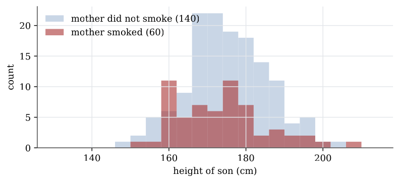
Two groups give two samples. Preferences for two colas, recorded as Bernoulli indicators in 100 boys and 100 girls, are independent \operatorname{Bern}(p_1) and \operatorname{Bern}(p_2) samples, or equivalently two independent binomial counts. Heights of men whose mothers did or did not smoke during pregnancy are two independent normal samples, and the comparison of interest is \mu_1-\mu_2. The intervals and tests for those comparisons are in Confidence intervals and Hypothesis tests. Worked numerical versions are in Estimation examples and Testing examples.
Every such model is an approximation. Heights are recorded on a discrete scale and cannot be negative, while a normal draw can be. The normal law is still useful when simulated samples look like the data and the mathematical summaries are tractable. A model that cannot reproduce the rough shape of the data is not a basis for a conclusion. Checking that shape is part of Descriptive statistics.
Observational studies and experiments
Data often arrive as a spreadsheet: one row per unit, one column per variable. Units are the people, plants, households, or objects that were measured.
Definition 1 (Observational study) In an observational study the investigator does not assign the conditions being compared. A survey is the usual case. Repeating the study would produce new values in every column, because a new set of units is encountered and nothing was fixed by design.
Definition 2 (Designed experiment) In a designed experiment some columns are controlled. Treatments are assigned to units, often at random, and those assignments stay the same if the measurements are repeated. The response column changes; the treatment column does not.
The variables one hopes to explain are the response, also called the outcome. The variables used to explain it are explanatory variables, also called covariates or factors. A randomised design assigns each unit one of a small number of treatments with equal probability. After a large enough randomisation, the treatment groups agree, before treatment, on the distribution of every variable, measured or not. A difference that then appears in the response is evidence about the treatments, not about who happened to land in which group.
Measurements vary for more than one reason. Most of the variation in heights is natural diversity between people, from genetics, diet and environment. Some is measurement error. Later models try to explain part of the variation by other variables, such as sex or shoe size. What no variable in the model explains is the residual variability, and a good model leaves little of it while still predicting new data well. One or more measurements are taken on each experimental unit: a person, a plant, a plot of land, a household, a star or a manufactured object.
Definition 3 (Randomised controlled trial) In a randomised controlled trial each experimental unit receives one of several treatments, chosen at random with equal probability, and one of the treatments is a control, such as the standard treatment or a placebo. The response is then compared between the treatment groups.
Definition 4 (Confounding variable) A confounding variable affects both the explanatory variable and the response, so that an association between those two can appear, disappear or reverse when the confounder is taken into account.
Taller people tend to have shorter hair. Within each sex there may be no relationship at all: women are on average shorter than men and on average have longer hair, and sex drives both. Sex confounds the comparison of height and hair length. In a well-run randomised experiment confounding cannot arise in this way, because the treatment groups have similar distributions of every variable.
Observational studies are retrospective when they analyse data that already exist, collected for some other purpose, and prospective when they are planned and the measurements follow. Neither assigns treatments. Many attributes cannot be assigned, for physical or ethical reasons: sex, age and beliefs are examples. A comparison between groups defined by such an attribute can show association with the response, but by itself not causation.
That is why a randomised comparison can support a causal sentence and an observational comparison usually cannot. In the smoking-and-height example the mothers were not assigned to smoke. A difference in sons’ heights is compatible with an effect of smoking and also with diet, income, or anything else that differs between the two groups of mothers. Randomisation is what blocks that reading.
Blinding keeps the assignment from leaking into the response. In a blind experiment the unit does not know which treatment it received. In a double-blind experiment the person who measures the response does not know either. A placebo, an inactive treatment that otherwise resembles the active one, is what makes that possible when the act of being treated itself changes the response.
Definition 5 (Blinding and placebo) In a blind experiment the units do not know which treatment they received. In a double-blind experiment the people who give the treatments and measure the responses do not know either. A placebo is a control treatment that resembles the active one in every manageable way but lacks the active ingredient.
Blinding matters because knowledge of the treatment can change the response. Patients given an inactive sugar pill sometimes report less pain; that is the placebo effect, and only a comparison against a placebo can separate it from the effect of the drug.
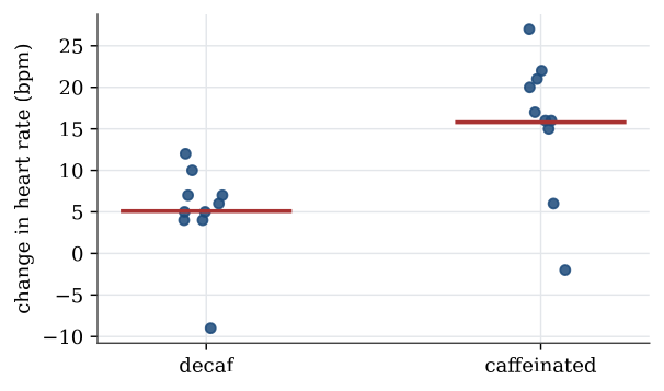
Example 1 (Alice’s caffeine experiment) Alice asks whether caffeinated cola raises the heart rate more than decaffeinated cola. She measures the heart rates of 20 friends, gives 10 of them 250 mL of caffeinated diet cola and 10 caffeine-free diet cola, waits half an hour, and measures again. The changes in beats per minute are
| Caffeinated | 17 | 22 | 21 | 16 | 6 | −2 | 27 | 15 | 16 | 20 |
| Decaf | 4 | 10 | 7 | −9 | 5 | 4 | 5 | 7 | 6 | 12 |
Question. Identify the response, the explanatory variable and the design choices, and summarise the data.
Solution. The experimental units are the 20 friends. The response is the change in heart rate, and the explanatory variable is caffeine, a factor with two levels. Several choices protect the comparison. Diet cola is compared with decaf diet cola because the two differ only in caffeine; regular and decaf regular cola also differ in sugar, energy and sodium. Half an hour is roughly the time caffeine takes to be absorbed. Choosing the 10 caffeine drinkers at random, rather than as, say, the 10 women, prevents a difference in heart rate from being a difference between the groups. Not telling the friends which drink they had, and ideally not telling whoever reads the pulse meter, prevents expectations from moving the response. Using friends at all limits the conclusion to people like Alice’s friends.
The decaf group’s mean change is 5.1 beats per minute and the caffeinated group’s is 15.8, a difference of 10.7. In a spreadsheet the data should be in standard form, one row per friend, with a column for the change and a column for the caffeine level:
alice <- data.frame(
  pb = c(17, 22, 21, 16, 6, -2, 27, 15, 16, 20, 4, 10, 7, -9, 5, 4, 5, 7, 6, 12),
  Caffeine = rep(c("Yes", "No"), each = 10)
)
tapply(alice$pb, alice$Caffeine, mean)
Whether a difference of 10.7 could easily arise by chance, with no effect of caffeine, is the question of the two-sample t test, worked in Testing examples.
A study that does not need every covariate recorded is one that randomised. Age, diet, and fitness still affect blood pressure, but if the drug and the control were assigned at random they are balanced across those variables, including the ones nobody wrote down. An observational study of the same question has to measure them, or the comparison stays confounded.
Sampling from a population
Most methods in this section assume a simple random sample. Collecting data costs time and money per unit, so the sampling design is usually a compromise between that cost and how representative the sample is.
Definition 6 (Simple random sample) A simple random sample of size n from a finite population of size N is drawn without replacement so that every subset of n members is equally likely to be the sample. In particular, every member has the same probability n/N of being included.
If each unit can be measured remotely, by phone or online, a simple random sample is easy to draw. Number the population and let the computer choose:
chosen <- sample(1:100000, 200)Each run gives a different set of 200 indices. The numbers come from a pseudorandom generator, which for this purpose behaves like true randomness; see Simulation.
When units must be visited in person, a simple random sample scattered over a whole country is slow and expensive. Two classic designs keep the randomness and cut the cost.
Definition 7 (Stratified and cluster sampling) In stratified sampling the population is split into subgroups called strata, and a simple random sample is drawn from each, usually of size nN_s/N for a stratum of size N_s. In cluster sampling the population is split into many small clusters, a few clusters are chosen at random, and every unit in each chosen cluster is measured, or a simple random sample is taken within it.
A stratum can be oversampled when it needs more precise estimates; stratifying needs accurate population counts for each stratum. Both designs weaken the independence of the observations a little, since units in one cluster or stratum share something the rest of the population does not, and that tends to raise the variance of estimates somewhat. Being able to afford more observations for the same cost usually more than makes up for it.
Example 2 (Sampling ten villages) A population lives in 10 small villages: 5 eastern villages of 50 people and 5 western villages of 100 people, so N=750. A sample of n=100 is wanted.
Question. How would a stratified sample and a cluster sample be drawn?
Solution. Stratify by east and west, of sizes 250 and 500. The eastern share is 100\times250/750=33.3, so take a simple random sample of 33 eastern villagers and 67 western ones. That will almost certainly reach every village, which is fair and representative but means a lot of travel.
For a cluster sample, make each eastern village a cluster of 50, and split each western village into two clusters of 50, giving 15 clusters. Choosing 2 clusters at random and measuring everyone in them gives the 100 observations with at most two villages visited, but most of the variety between villages is never seen. A middle course chooses 4 clusters and takes a random half of each, 4\times25=100, at the cost of visiting up to four villages. Stratifying into east and west first and then clustering within each would guarantee both regions appear.
Many data are collected in ways far from random. A convenience sample takes whoever is available, and generalises only if the available units resemble the population. A self-selected sample takes whoever chooses to take part, as in a television phone-in poll; it rarely represents even the show’s viewers, and a keen caller may vote twice. In both, units are not sampled independently with equal probability, which biases estimates, and a larger sample of the same kind does not remove the bias.
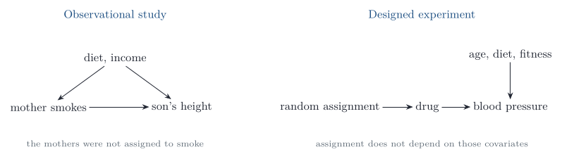
Write down the response, the explanatory variables, and whether the explanatory variables were assigned or only observed. Random assignment is what turns a difference between groups into evidence about the treatment.
Questions on this topic
Open a question to attempt it. Its worked answer is folded away at the bottom of the page.
What links here
Pages (5)
- Descriptive statistics — via Studies, data, and evidence, designed experiment
- Testing examples — via Alice’s caffeine experiment
- Analysis of variance examples — via placebo, designed experiment
- Bayesian foundations — via randomised experiment, Studies, data, and evidence
- Marginal models, and two responses at once — via confounded
Questions and answers (3)