Smooth means
Part of Smoothing · 5 questions on this topic · What links here
Smooth means
| Part | Smoothing |
| Chapter | 1 of 2 in this part |
| Next | Additive smooths |
| Questions | 5 |
| Figures | 3 |
A coefficient is worth having when you can say what a unit change does. In a linear model, \beta_j is the change in the mean. In a log-linear model, e^{\beta_j} is the multiplicative change. In a logit model, \beta_j is the change in log-odds. Powers, logarithms, and products of covariates are still linear in the parameters, and they are still GLMs. The limitation is that you had to name the function before you saw the curve.
Sometimes nothing in the science names it. Dosage and exposure want a logarithm for a reason we have already used. A rate wants a log link because the natural parameter said so. A lidar return, plotted against distance, does not offer you that sentence in advance.
Lidar
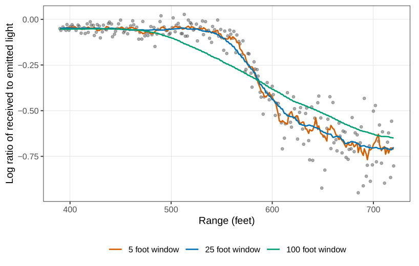
Ruppert, Wand, and Carroll’s lidar data take Y to be the log ratio of received light to emitted light, and x the range in feet. A perfect return would sit at 0. Some points sit above 0 because the room is not dark: the sensor records the laser plus whatever else is shining. Out to roughly 500 or 550 feet the mean is flat. Past that threshold it drops, sharply, and the scatter widens as the mean falls. A laser gets weaker with distance and it gets noisier. The variance is a GLM problem, and we already know how to write \mathrm{Var}=\phi V(\mu). The mean is not a quadratic we would have written down before seeing the plot, and we would not want to have to name the threshold.
A moving window is the first smoother you are likely to have seen. In Figure 1, averaging within \pm 5 feet leaves a noisy curve. Within \pm 25 feet it is calmer but still jagged on the drop. Within \pm 100 feet it is smooth and it has smeared the drop. A single window width cannot be wide where the noise is large and narrow where the signal is sharp. The window also ignores the mean-variance relationship, so it oversmooths the precise part of the curve and undersmooths the noisy part. The penalty has to live on the likelihood scale, where a GLM already knows that a residual at a large mean is not the same as a residual at a small one.
A roughness penalty
Green and Silverman’s formulation is the clean one, even though we no longer compute it with a knot at every x. Keep the exponential family. Replace the linear predictor by an unknown smooth function g(x), and keep the canonical link, so the mean is -c'(g(x)). For the normal that is g(x) itself. For the Poisson it is \exp(g(x)), which stays positive whatever g does. For the Bernoulli it is the expit of g(x), which stays inside (0,1). For the gamma the canonical choice is 1/g(x), and that still requires g not to change sign. You may use a log link for the gamma instead. Nothing forces the canonical link once you have decided the mean is smooth rather than linear.
Maximise the log-likelihood and charge for curvature: \sum_{i=1}^n\bigl\{y_i g(x_i)-c(g(x_i))\bigr\} -\frac{\lambda}{2}\int \{g''(x)\}^2\,\mathrm{d}x. The first piece wants g to pass through the data. The integral of the squared second derivative is large when the curve turns often. A straight line has second derivative zero and pays nothing. A sine wave pays on every oscillation. \lambda is the exchange rate between fidelity and smoothness. The half is cosmetic: for the normal likelihood it cancels the usual factor of one half.
The maximiser, for any fixed \lambda, is a cubic spline with a knot at each distinct x_i. Inside each interval the function is a cubic. At each knot the function, the first derivative, and the second derivative agree from the left and the right. Your eye can see those three. It cannot see a jump in the third derivative, which is why a cubic, rather than a higher piecewise polynomial, is the one this penalty produces.
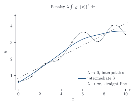
Putting a knot at every x_i is expensive, and \lambda itself changes meaning when you change the likelihood. In practice we use a smaller set of knots, ten equally spaced between the smallest and largest x being the usual default, or knots at the deciles if the x values pile up at one end. More knots are available when the sample is in the thousands. And we do not quote \lambda. Cross-validation hides a fraction of the sample, fits on the rest, and scores the hidden points, rotating which fraction is hidden. The software reports the smoothness as an equivalent degrees of freedom: the polynomial degree the curve is about as flexible as. As \lambda\to\infty that degrees of freedom falls to 1, a straight line, which is the ordinary GLM. As \lambda\to 0 the fit interpolates, and if no x values are tied it interpolates perfectly. Interpolation fits noise. It does not predict the next point.
Kyphosis and age
Eighty-one children were followed after spinal surgery to see whether kyphosis, a forward bend in the spine, was still present. Age is recorded in months, from infancy out to about 200 months. The ones and zeros rise through the middle ages and fall again. A logistic regression with age as a linear predictor can only ever increase, or only ever decrease. It cannot come back down. So keep the logistic mean, and let the inside be a smooth function centred at zero:
\mathrm{P}(\text{kyphosis}\mid \text{age})
=\frac{\exp\{\beta_0+g(\text{age})\}}{1+\exp\{\beta_0+g(\text{age})\}},
where g is constrained to average zero so that \beta_0 is the log-odds at the centre of the age effect. In mgcv,
need <- function(pkg) {
  if (!requireNamespace(pkg, quietly = TRUE)) {
    install.packages(pkg, repos = "https://cloud.r-project.org")
  }
  suppressPackageStartupMessages(library(pkg, character.only = TRUE))
}
need("mgcv")
need("rpart")
data(kyphosis, package = "rpart")
kyphosis$Kyphosis <- as.numeric(kyphosis$Kyphosis == "present")
fit <- gam(Kyphosis ~ s(Age), family = binomial, data = kyphosis)
summary(fit)
s(Age) asks for the smooth. Knots and \lambda are chosen by cross-validation. The plotted smooth is labelled with equivalent degrees of freedom 2.22: more flexible than a quadratic, short of a cubic, and not itself a polynomial of degree 2.22. It is a piecewise cubic whose overall budget of wiggliness is 2.22. The intercept is -1.51 (z=-4.78), so at the centre of g the odds are e^{-1.51}. The smooth term has
\mathrm{edf}=2.22,\qquad \chi^2=6.69,\qquad p=0.071.
The equivalent degrees of freedom and the intercept -1.51 are what the code prints. The chi-squared statistic moves with the version of mgcv: one printout was 6.69 with p=0.071, and mgcv 1.8 reports about 6.36 with p=0.076. Either reading is the same decision.
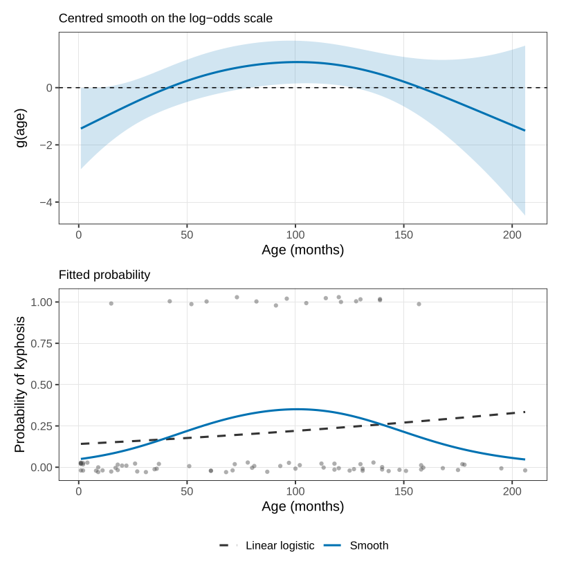
In Figure 3 a horizontal line at zero just about stays inside the band, and it just about fails to. We do not have a hard rule at 0.05. We keep age. The fitted probability, the expit of \beta_0+g, rises and then falls. That graph is the answer to “how does kyphosis depend on age?”. There is no unit-change sentence, and that is the price of not having specified the shape in advance.
The substantive reading we would offer, cautiously, is a mixture of biology and of who is sent to surgery. Very young children are operated on because the problem is serious, and they also recover more readily. Older adolescents are often milder cases, chosen for correction once the skeleton is more settled. The ages in the middle are the ones whose surgery was delayed and whose bones were no longer infant bones. You cannot randomise the age at which an elective operation happens. The curve is a description of this sample, not a pure age effect.
Number of vertebrae operated on, and where on the spine the operation started, are in the same data set. They are the next chapter. A smooth of age alone is the model this chapter stops on.
In the penalised criterion, what does the fitted g become as \lambda\to\infty, and what does it become as \lambda\to 0 if all the x_i are distinct?
The kyphosis smooth has equivalent degrees of freedom 2.22 and a p-value of about 0.07. Say what each of those numbers is measuring, and why a logistic regression that is linear in age cannot reproduce the shape in the plot.
Questions on this topic
Open a question to attempt it. Its worked answer is folded away at the bottom of the page.
What links here
Questions and answers (1)