Testing examples
Part of Data analysis · 6 questions on this topic · What links here
Testing examples
| Part | Data analysis |
| Chapter | 5 of 9 in this part |
| Previous | Estimation examples |
| Next | Analysis of variance examples |
| Questions | 6 |
| Figures | 1 |
The definitions of a null hypothesis, a test statistic, a p-value, size and power are in Hypothesis tests. This page runs the standard tests on data in R and reads the output. The p-value R prints is the one defined there: the probability, if the null hypothesis were true, of a statistic at least as extreme as the one observed. It is not the probability that the null hypothesis is true; that calculation is in Bayesian hypotheses and model comparison.
Power by simulation
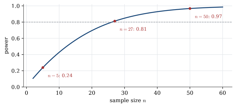
The power of a test is the probability that it rejects when the null hypothesis is false. For most tests it can be computed by formula, but simulation makes the idea concrete: generate many data sets from a chosen alternative, run the test on each, and count the rejections.
Example 1 (Simulating the power of a t test) A one-sample t test of H_0:\mu=0 against H_1:\mu>0 is run at level 0.05 on n observations.
Question. What is its power if the data are really \operatorname{N}(1,2^2), with n=5 and with n=50?
Solution.
R <- 1e5; n <- 5; mu <- 1; sigma <- 2
pval <- replicate(R, {
  x <- rnorm(n, mean = mu, sd = sigma)
  1 - pt(mean(x) / (sd(x) / sqrt(n)), df = n - 1)
})
mean(pval < 0.05)                      # about 0.24
power.t.test(n = 5, delta = 1, sd = 2, sig.level = 0.05,
             type = "one.sample", alternative = "one.sided")$power   # 0.239
With five observations the test detects a mean of 1 only 24% of the time. With n=50 the power is 0.967. The power depends on \mu and \sigma only through their ratio \mu/\sigma, here 1/2, together with n and the level. A power calculation of this kind, using a guess at \sigma from a pilot study, is how a sample size is chosen before the data are collected.
One proportion: exact or approximate
Example 2 (A new sweetener) Ten people each taste two yoghurts, one with an old sweetener and one with a new one. Eight prefer the new one.
Question. Test whether the new sweetener is preferred, exactly and by the normal approximation.
Solution. Let X\sim\operatorname{Bin}(10,p) be the number preferring the new yoghurt, and test H_0:p=0.5 against H_1:p>0.5. The exact binomial test has p-value \mathbb{P}(X\ge8)=0.0547:
binom.test(x = 8, n = 10, p = 0.5, alternative = "greater")
# number of successes = 8, number of trials = 10, p-value = 0.05469
The normal approximation uses z=(0.8-0.5)/\sqrt{0.5\times0.5/10}=1.897, with p-value 0.0289:
prop.test(x = 8, n = 10, p = 0.5, alternative = "greater", correct = FALSE)$p.value
# 0.02889
The two p-values differ by a factor of two, and they fall on opposite sides of 0.05. Ten observations are too few for the central limit theorem, so the exact test is the one to report. For small samples use binom.test.
Two independent samples
Example 3 (Alice’s caffeine test) The heart-rate changes in Alice’s caffeine experiment were 17, 22, 21, 16, 6, −2, 27, 15, 16, 20 for the caffeinated group and 4, 10, 7, −9, 5, 4, 5, 7, 6, 12 for decaf.
Question. Is there evidence that caffeine increases the heart rate?
Solution. Model the two groups as independent normal samples with means \mu_1 (caffeinated) and \mu_2 (decaf), and test H_0:\mu_1=\mu_2 against H_1:\mu_1>\mu_2.
caf   <- c(17, 22, 21, 16, 6, -2, 27, 15, 16, 20)
decaf <- c(4, 10, 7, -9, 5, 4, 5, 7, 6, 12)
t.test(caf, decaf, alternative = "greater")
# t = 3.3752, df = 15.74, p-value = 0.001966
t.test(caf, decaf, alternative = "greater", var.equal = TRUE)$p.value   # 0.001686
The difference in means is 10.7 beats per minute. R’s default is the Welch test, with 15.7 effective degrees of freedom and p-value 0.002; the pooled two-sample t test gives p=0.0017. Either way, a difference this large would be very unlikely without an effect of caffeine. Because the drink was assigned at random, the evidence is evidence that caffeine raises the heart rate, for people like Alice’s friends. The two-sided 95% Welch interval for the effect is (4.0,\ 17.4) beats per minute: an effect is clear, its size is not pinned down.
Paired samples
Example 4 (Two labs on the same patients) Two labs measure the same quantity on the same 15 patients.
lab1 <- c(22, 18, 28, 26, 13, 8, 21, 26, 27, 29, 25, 24, 22, 28, 15)
lab2 <- c(25, 21, 31, 27, 11, 10, 25, 26, 29, 28, 26, 23, 22, 25, 17)
Question. Do the labs differ on average?
Solution. The two columns are not independent: a patient with a low value gets it from both labs, as patient 6 does with 8 and 10. So analyse the differences D_i=X_i-Y_i as one sample, D_i\sim\operatorname{N}(\delta,\sigma^2), and test H_0:\delta=0 against \delta\neq0:
t.test(lab1, lab2, paired = TRUE)
# t = -1.7618, df = 14, p-value = 0.0999
The mean difference is -0.93 with standard deviation 2.05, so t=-0.93/(2.05/\sqrt{15})=-1.76 and p=0.10. There is weak evidence, at most, that lab 2 reads higher. Ignoring the pairing and running a two-sample test gives t=-0.42 and p=0.68: the large differences between patients swamp the small, consistent difference between labs. Pairing removes the patient effect.
Two proportions
For two independent binomial counts, prop.test with two counts tests H_0:p_1=p_2 with the two-proportion z test; its printed statistic is the square of z, a chi-squared statistic on one degree of freedom. For 40 left-wing viewers out of 70 on one channel against 50 out of 100 on another,
prop.test(c(40, 50), c(70, 100), alternative = "greater", correct = FALSE)
# X-squared = 0.8433, df = 1, p-value = 0.1792
and \sqrt{0.8433}=0.918 is the z statistic. There is no evidence that the first channel’s audience is more left-wing.
State the model and the hypotheses, then let R compute the statistic and the p-value. Use the exact binomial test for a small count, pair measurements made on the same unit, and plan the sample size from the power, not after the data are in.
Questions on this topic
Open a question to attempt it. Its worked answer is folded away at the bottom of the page.
| Question | Answer |
|---|---|
| Caffeine in a cola | ✓ |
| A later poll on leaving | ✓ |
| Steel rod diameters | ✓ |
| A shuffling machine | ✓ |
| Two proportions | ✓ |
| Home-ground wins | ✓ |
What links here
Pages (3)
- Studies, data, and evidence — via Testing examples
- Using R — via Testing examples
- Bayesian hypotheses and model comparison — via Testing examples