Confidence intervals
Part of Statistical inference · 6 questions on this topic · What links here
Confidence intervals
| Part | Statistical inference |
| Chapter | 3 of 7 in this part |
| Previous | Estimation |
| Next | Hypothesis tests |
| Questions | 6 |
| Definitions | Confidence interval · Pivot · Pooled variance · Wald interval |
| Results | One-sample t pivot · Two-sample t pivot · Variance-ratio F pivot |
| Figures | 2 |
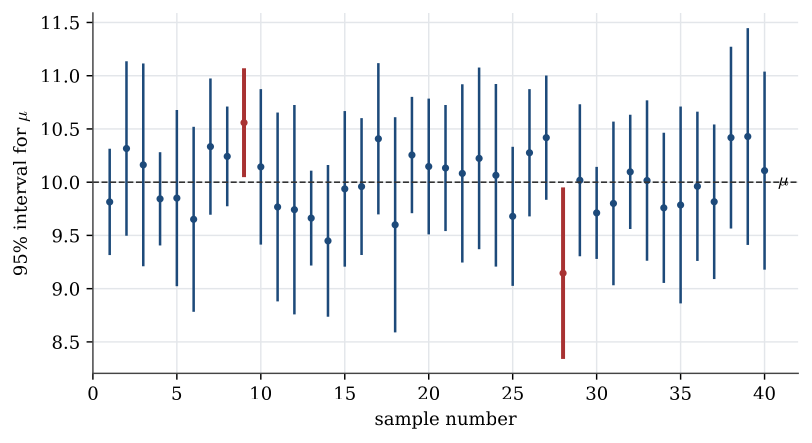
A point estimate does not say how far it might fall from the parameter. A confidence interval attaches a long-run coverage probability to a random interval built from the sample. After the sample is observed the endpoints are numbers. The confidence, say 95%, is a property of the procedure that produced them, not a probability that the parameter lies in that particular interval.
That last distinction is the same one drawn for a credible interval. A credible interval puts the probability on the parameter, given the data. A confidence interval puts the probability on the interval, given the parameter.
The normal, chi-squared, t and F laws used below are defined in Statistical inference, together with the normal sample theorem that links them to a sample. The binomial intervals rest on the central limit theorem.
From a standard error to an interval
A company introduced new safety measures. In the 50 months since, lost working hours averaged 91 per month, with bias-corrected sample standard deviation 14.1. In the 50 months before, they averaged 108, with standard deviation 14.3. The estimate of the change in mean is 91-108=-17 hours per month. How accurate is it?
Model the two runs of months as independent samples, with means \mu_1 and \mu_2 and a common variance \sigma^2. The estimator \overline X_1-\overline X_2 is unbiased for \mu_1-\mu_2, with variance
\operatorname{Var}(\overline X_1-\overline X_2)=\frac{\sigma^2}{50}+\frac{\sigma^2}{50}=\frac{\sigma^2}{25}.
Estimating \sigma^2 by the pooled variance s_p^2=(49\times14.1^2+49\times14.3^2)/98=14.20^2 gives a standard error of 14.20/5=2.84. A common way to report this is -17\pm2.84, or -17\pm2\times2.84.
What probability goes with “estimate plus or minus a standard error”? Take the simplest case, X_1,\ldots,X_n independent and \operatorname{N}(\mu,1). Then \sqrt n(\overline X-\mu) is standard normal, and
\mathbb{P}\bigl(\overline X-n^{-1/2}<\mu<\overline X+n^{-1/2}\bigr)=\mathbb{P}\bigl(-1<\sqrt n(\overline X-\mu)<1\bigr)=2\Phi(1)-1=0.683.
Plus or minus one standard error covers \mu only 68% of the time. Plus or minus two covers it with probability 2\Phi(2)-1=0.954. Choosing the multiplier is choosing the coverage.
Coverage
Definition 1 (Confidence interval) Let L and U be statistics. The random interval (L,U) is a confidence interval for \theta with confidence 1-\alpha when
\mathbb{P}_\theta(L<\theta<U)=1-\alpha
for every \theta. A one-sided interval leaves one endpoint infinite.
The observed interval (l,u), computed from the data, is still called the confidence interval. Smaller \alpha means a wider interval, and a very wide interval says little. The usual choices are 0.01, 0.05 and 0.10, that is 99%, 95% and 90% confidence. When the coverage holds only for large samples, the interval is approximate.
Suppose a 90% interval for \mu comes out as (9.5,10.5). It is tempting to write \mathbb{P}(9.5<\mu<10.5)=0.9, but \mu is a fixed number, so that probability is either 0 or 1, and which one is unknown. The 0.9 belongs to the random interval (L,U) before the data arrive. An urn holds 90 white balls and 10 black. Draw one without looking. You are fairly sure it is white, and you hold it in a closed hand. That is the right degree of confidence that (9.5,10.5) contains \mu.
Definition 2 (Pivot) A pivot is a function h({\boldsymbol{X}};\theta) of the data and the parameter whose distribution does not depend on any unknown parameter.
Every interval in this chapter is built the same way. Find a pivot. Choose its quantiles h_{\alpha/2} and h_{1-\alpha/2}, so that
\mathbb{P}\bigl(h_{\alpha/2}<h({\boldsymbol{X}};\theta)<h_{1-\alpha/2}\bigr)=1-\alpha.
Rearrange the inequality to isolate \theta. The rearrangement does not change the event, so the coverage is still 1-\alpha. The pivot must not depend on unknown parameters, or its quantiles cannot be computed. That is why the t statistic, which replaces \sigma by s, is a pivot, and \sqrt n(\overline X-\mu)/\sigma with unknown \sigma is not.
One normal sample
Let X_1,\ldots,X_n be independent and \operatorname{N}(\mu,\sigma^2).
If \sigma is known,
Z=\frac{\overline X-\mu}{\sigma/\sqrt n}
is standard normal. Writing z_{1-\alpha/2} for the standard normal quantile of order 1-\alpha/2,
\overline X\pm z_{1-\alpha/2}\,\frac{\sigma}{\sqrt n}
is a confidence interval for \mu with confidence 1-\alpha. For 95%, z_{0.975}=1.960.
If \sigma is unknown, replace it by s. The pivot is no longer normal.
Theorem 1 (One-sample t pivot) If X_1,\ldots,X_n are independent and \operatorname{N}(\mu,\sigma^2), then
T=\frac{\overline X-\mu}{s/\sqrt n}
has a Student t distribution with n-1 degrees of freedom. A Student variable with m degrees of freedom is Z/\sqrt{V/m} where Z is standard normal, V is chi-squared with m degrees of freedom, and Z and V are independent.
To see this, divide top and bottom by \sigma/\sqrt n:
T=\frac{(\overline X-\mu)/(\sigma/\sqrt n)}{\sqrt{\dfrac{(n-1)s^2/\sigma^2}{n-1}}}=\frac{Z}{\sqrt{V/(n-1)}}.
By the normal sample theorem, Z is standard normal, V=(n-1)s^2/\sigma^2 is \chi^2_{n-1}, and they are independent, because Z depends on \overline X alone and V on s^2 alone. The unknown \sigma has cancelled, so T is a pivot.
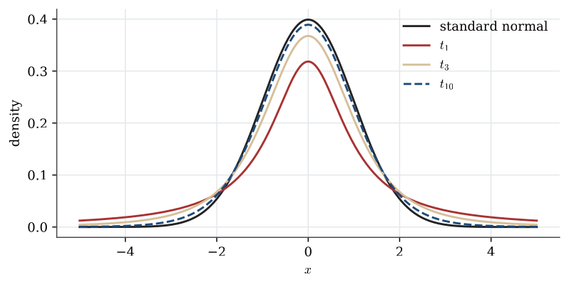
Placing T between \pm t_{n-1;1-\alpha/2} and solving for \mu gives the interval
\overline X\pm t_{n-1;\,1-\alpha/2}\,\frac{s}{\sqrt n},
where t_{m;q} is the quantile of order q of the t distribution with m degrees of freedom. For large n this quantile is close to the corresponding normal quantile, because s is then close to \sigma.
Example 1 (Household fuel spending) An oil company samples 51 households at random from a city. They spent on average \overline x=1136 dollars a year on petrol and heating oil, with bias-corrected standard deviation s=178 dollars.
Question. Give a 95% confidence interval for the mean spending \mu in the city, and say what the model assumes.
Solution. Model the spending of the 51 households as a random sample from \operatorname{N}(\mu,\sigma^2), both unknown. Random selection justifies independence and a common distribution. Normality is an assumption; with n=51 the central limit theorem makes it matter little for an interval about the mean. With t_{50;0.975}=2.009, the standard error is 178/\sqrt{51}=24.93, and
1136\pm2.009\times24.93=1136\pm50.1=(1085.9,\ 1186.1).
A variance
The variance uses the chi-squared pivot (n-1)s^2/\sigma^2, which is \chi^2_{n-1} by the normal sample theorem. Writing \chi^2_{m;q} for its quantile of order q,
\mathbb{P}\Bigl(\chi^2_{n-1;\,\alpha/2}<\frac{(n-1)s^2}{\sigma^2}<\chi^2_{n-1;\,1-\alpha/2}\Bigr)=1-\alpha.
Solving for \sigma^2 gives the confidence interval
\left(\frac{(n-1)s^2}{\chi^2_{n-1;\,1-\alpha/2}},\;\frac{(n-1)s^2}{\chi^2_{n-1;\,\alpha/2}}\right).
The upper quantile sits in the lower endpoint, because the pivot has \sigma^2 in the denominator. The chi-squared law is skewed, so the interval is not symmetric about s^2. An interval for \sigma is found by taking square roots of both endpoints; a monotone function carries the coverage with it.
Example 2 (Aspirin tablet weights) A label states that tablet weights have standard deviation 1.0 mg. A sample of 25 tablets has s=1.3 mg.
Question. Give 95% confidence intervals for \sigma^2 and for \sigma, assuming normal weights. Is the label believable?
Solution. With 24 degrees of freedom, \chi^2_{24;0.025}=12.40 and \chi^2_{24;0.975}=39.36. Since (n-1)s^2=24\times1.69=40.56,
\left(\frac{40.56}{39.36},\ \frac{40.56}{12.40}\right)=(1.03,\ 3.27)
for \sigma^2, and (1.02,\ 1.81) mg for \sigma. The interval for \sigma excludes the stated 1.0 mg, so the data cast doubt on the label at the 95% level.
Two normal samples
Let the first sample have size n_1, mean \overline X_1 and variance s_1^2, and the second sample size n_2, mean \overline X_2 and variance s_2^2. The samples are independent, the first is \operatorname{N}(\mu_1,\sigma_1^2), and the second is \operatorname{N}(\mu_2,\sigma_2^2).
A difference of means
The construction is like the one-sample case, with one extra assumption: the two variances are equal, \sigma_1^2=\sigma_2^2=\sigma^2. Then
\frac{(\overline X_1-\overline X_2)-(\mu_1-\mu_2)}{\sigma\sqrt{1/n_1+1/n_2}}
is standard normal, and the common variance is estimated by pooling.
Definition 3 (Pooled variance) For two independent samples assumed to share a variance \sigma^2, the pooled sample variance is
s_p^2=\frac{(n_1-1)s_1^2+(n_2-1)s_2^2}{n_1+n_2-2}.
It is unbiased for \sigma^2, and (n_1+n_2-2)s_p^2/\sigma^2 is \chi^2_{n_1+n_2-2}.
The pooled variance weights each sample variance by its degrees of freedom. The chi-squared statement holds because (n_1-1)s_1^2/\sigma^2 and (n_2-1)s_2^2/\sigma^2 are independent \chi^2_{n_1-1} and \chi^2_{n_2-1} variables, and independent chi-squared variables add their degrees of freedom.
Theorem 2 (Two-sample t pivot) For two independent normal samples with a common variance,
T=\frac{(\overline X_1-\overline X_2)-(\mu_1-\mu_2)}{s_p\sqrt{1/n_1+1/n_2}}
has a t distribution with n_1+n_2-2 degrees of freedom.
The proof is the one-sample argument again. The numerator over \sigma\sqrt{1/n_1+1/n_2} is standard normal, the pooled chi-squared variable is (n_1+n_2-2)s_p^2/\sigma^2, and the two are independent because each sample mean is independent of its own sample variance and the samples are independent of each other. The resulting interval for \mu_1-\mu_2 is
\overline X_1-\overline X_2\pm t_{n_1+n_2-2;\,1-\alpha/2}\;s_p\sqrt{\frac1{n_1}+\frac1{n_2}}.
For the safety measures, n_1=n_2=50, the estimate is -17, the standard error is 2.84, and t_{98;0.975}=1.984. The 95% interval is
-17\pm1.984\times2.84=-17\pm5.64=(-22.6,\ -11.4).
It lies wholly below zero. The interval -17\pm2.84, one standard error each side, would have coverage of only about 68%.
A ratio of variances
The pooled interval is valid only if the variances are equal. That can be checked with an interval for \sigma_1^2/\sigma_2^2, and seeing whether it contains 1.
Theorem 3 (Variance-ratio F pivot) For two independent normal samples,
\frac{s_1^2/\sigma_1^2}{s_2^2/\sigma_2^2}
has the F distribution with (n_1-1,\,n_2-1) degrees of freedom.
Write U=(n_1-1)s_1^2/\sigma_1^2 and V=(n_2-1)s_2^2/\sigma_2^2. These are independent \chi^2_{n_1-1} and \chi^2_{n_2-1} variables, and the ratio is \{U/(n_1-1)\}/\{V/(n_2-1)\}, which is the definition of F_{n_1-1,n_2-1}. Placing the pivot between its quantiles and using 1/F_{m_1,m_2;\,\alpha/2}=F_{m_2,m_1;\,1-\alpha/2} gives the interval
\left(\frac{1}{F_{n_1-1,n_2-1;\,1-\alpha/2}}\,\frac{s_1^2}{s_2^2},\ \ F_{n_2-1,n_1-1;\,1-\alpha/2}\,\frac{s_1^2}{s_2^2}\right).
For the safety measures, s_1^2/s_2^2=14.1^2/14.3^2=0.972 and F_{49,49;0.975}=1.762, so the 95% interval for \sigma_1^2/\sigma_2^2 is (0.552,\ 1.713). It contains 1, so there is no reason at the 5% level to doubt the equal-variance assumption behind the pooled interval.
A proportion
Let X\sim\operatorname{Bin}(n,p) and \widehat p=X/n. An exact interval is awkward because the binomial law is discrete. For large n the central limit theorem gives
\frac{\widehat p-p}{\sqrt{p(1-p)/n}}\approx\operatorname{N}(0,1),
so \mathbb{P}(-z_{1-\alpha/2}<(\widehat p-p)/\sqrt{p(1-p)/n}<z_{1-\alpha/2})\approx1-\alpha. Solving for p leaves p inside the standard error. For large n, \widehat p is close to p, and replacing the unknown standard error by \sqrt{\widehat p(1-\widehat p)/n} produces an interval whose ends depend only on the data.
Definition 4 (Wald interval) For X\sim\operatorname{Bin}(n,p) with \widehat p=X/n, the Wald interval with approximate confidence 1-\alpha is
\widehat p\pm z_{1-\alpha/2}\sqrt{\frac{\widehat p(1-\widehat p)}{n}}.
It is an approximation. It behaves badly when n is small or \widehat p is near 0 or 1, because the estimated standard error is then a poor stand-in and the normal shape has not set in. At \widehat p=0 it collapses to a single point. A common rule is to use it only when n\widehat p and n(1-\widehat p) are both at least 5. It also models the sample as independent draws: a poll with refusals or untruthful answers has errors no interval formula can see.
For two independent samples the same approximation applies to \widehat p_1-\widehat p_2, whose variance is the sum of the two variances. The interval is
\widehat p_1-\widehat p_2\pm z_{1-\alpha/2}\sqrt{\frac{\widehat p_1(1-\widehat p_1)}{n_1}+\frac{\widehat p_2(1-\widehat p_2)}{n_2}}.
Example 3 (Nightmares in two groups) Of 160 men, 55 report frequent nightmares; of 192 women, 60 do.
Question. Give an approximate 95% confidence interval for the difference p_1-p_2 in the population proportions, and interpret it.
Solution. \widehat p_1=55/160=0.344 and \widehat p_2=60/192=0.313, a difference of 0.031. The standard error is
\sqrt{\frac{0.344\times0.656}{160}+\frac{0.313\times0.688}{192}}=0.0503,
so the interval is 0.031\pm1.96\times0.0503=(-0.067,\ 0.130). It contains 0. The data are consistent with no difference between men and women, and also with a difference of several percentage points either way.
How large a sample?
For a normal mean with known \sigma, the half-width of the interval is E=z_{1-\alpha/2}\,\sigma/\sqrt n. Solving for n, a half-width of at most E needs
n\ge\Bigl(\frac{z_{1-\alpha/2}\,\sigma}{E}\Bigr)^2.
Halving the half-width needs four times the sample. For a proportion the same calculation with \sigma^2=p(1-p)\le1/4 gives the conservative n\ge z_{1-\alpha/2}^2/(4E^2). A poll accurate to \pm3 percentage points with 95% confidence needs about 1.96^2/(4\times0.03^2)\approx1068 people, whatever the size of the population.
A confidence interval is a pivot solved for the parameter. The coverage probability is computed before the data are seen, over all the samples that might have been drawn. The numerical interval reported afterwards is not assigned that probability.
Questions on this topic
Open a question to attempt it. Its worked answer is folded away at the bottom of the page.
What links here
Pages (8)
- Statistical inference — via confidence interval
- Estimation — via pivots
- Hypothesis tests — via pivots, confidence intervals, pooled variance, confidence interval
- Linear regression — via confidence interval, pivot
- Studies, data, and evidence — via Confidence intervals
- Descriptive statistics — via confidence interval
- Estimation examples — via confidence interval, Confidence intervals, Wald interval
- Bayesian foundations — via confidence interval
Questions and answers (24)
- Which of these are statistics? (answer) · A proportion in a poll · The interval for a normal mean · Lost hours after a safety programme · Checking equal variances · Sizing a poll · How much do the ads explain? · Two groups (answer) · Ten normal observations · Narrowing a pilot interval · Printer paper · Hours of sleep · A difference of proportions · Variance of a fill volume · A later poll on leaving · Two proportions · Rain, food, and orange yield · How far sharks swim · Q3 · Q16 · Q25 · Q41 (answer) · Question 9 · C6
See also
- Articles from this chapter: Confidence interval · Pivot · One-sample t pivot · Pooled variance · Two-sample t pivot · Variance-ratio F pivot · Wald interval
- All statistical inference chapters
- Glossary and index
- Distribution sheet and formula lookup