Hypothesis tests
Part of Statistical inference · 6 questions on this topic · What links here
Hypothesis tests
| Part | Statistical inference |
| Chapter | 4 of 7 in this part |
| Previous | Confidence intervals |
| Next | Chi-squared tests |
| Questions | 6 |
| Definitions | Null and alternative hypotheses · Critical region · p-value · Type I and type II errors · Neyman–Pearson approach · Power function · One-sample t test · Two-sample t test · F test for equal variances · Binomial test · Two-proportion z test · Sign test |
| Figures | 3 |
A test asks whether the data would be surprising if a stated hypothesis were true. The probability in that question is computed under the hypothesis, before any probability is placed on the hypothesis itself. Putting probability on the hypotheses, and comparing them by a Bayes factor, is Bayesian hypotheses and model comparison. The p-value defined here is not that probability.
The pivots are the same ones used for confidence intervals: the normal, t, chi-squared, F and binomial laws, with the central limit theorem supplying the approximate normal tests.
Chance or an effect?
Systolic blood pressure among men aged 35 to 44 has mean 127 and standard deviation 7. A sample of 101 diabetic men has mean blood pressure 130. Is that evidence that diabetic men differ?
Ask how likely a sample mean this far from 127 would be if diabetic men were like everyone else. Under that supposition, model the readings as independent \operatorname{N}(127,7^2), so \overline X\sim\operatorname{N}(127,49/101) and
\mathbb{P}(\overline X\ge130)=\mathbb{P}\Bigl(Z\ge\frac{130-127}{\sqrt{49/101}}\Bigr)=\mathbb{P}(Z\ge4.31)=8.3\times10^{-6}.
An event that improbable has happened. Either something very unlikely occurred, or the supposition is wrong. The data are strong evidence that diabetic men differ.
Last season 60% of a tennis player’s first serves went in. After coaching, 13 of 15 go in. Suppose nothing changed, so the count is X\sim\operatorname{Bin}(15,0.6). Then
\mathbb{P}(X\ge13)=\sum_{k=13}^{15}\binom{15}{k}0.6^k\,0.4^{15-k}=0.0271.
That is small, though far less extreme than the blood-pressure case. There is reasonable evidence that the serve has improved.
Both examples follow one pattern. To show that an effect exists, show that something has happened which would be very unlikely if it did not.
The ingredients
The model is a random sample, or a count, whose distribution depends on \theta. The model must leave \theta free. In the blood-pressure example the model is X_i independent \operatorname{N}(\mu,7^2) with \mu unknown; setting \mu=127 in the model would assume the answer.
Definition 1 (Null and alternative hypotheses) The null hypothesis H_0 and the alternative hypothesis H_1 are two disjoint statements about the parameter, H_0:\theta\in\Theta_0 and H_1:\theta\in\Theta_1. H_0 is the statement being tested, often a single value \theta_0. H_1 is the claim the test is trying to detect.
The null is rejected only on strong evidence, so the claim of interest goes in the alternative. For the blood pressures, H_0:\mu=127 against H_1:\mu\neq127. For the serves, H_0:p=0.6 against H_1:p>0.6. An alternative of the form \theta\neq\theta_0 is two-sided; \theta>\theta_0 and \theta<\theta_0 are one-sided.
A test statistic T is a statistic that is sensitive to the difference between H_0 and H_1. Like any statistic, it must not contain unknown parameters. Its null distribution is the distribution of T when H_0 is true. In the blood-pressure example \overline X, \overline X-127 and \sum X_i all work, because each carries the same information and each has a known null distribution.
Definition 2 (Critical region) A critical region C is a set of values of the test statistic. The test rejects H_0 when T\in C. A right-sided region is [c,\infty), a left-sided region is (-\infty,c], and a two-sided region is (-\infty,c_1]\cup[c_2,\infty).
The shape of C follows from H_1. For the blood pressures, a mean much larger or much smaller than 127 is evidence against H_0, so C is two-sided. For the serves, only a large count is evidence for improvement, so C=\{c,\ldots,15\}.
Definition 3 (p-value) The p-value of an observed statistic t is the probability, under H_0, that T is at least as extreme as t, in the direction of H_1. For a two-sided normal or t statistic it is twice the one-sided tail probability beyond |t|.
Concretely, for a left-sided test p=\mathbb{P}_{H_0}(T\le t), for a right-sided test p=\mathbb{P}_{H_0}(T\ge t), and for a two-sided test
p=\min\{2\mathbb{P}_{H_0}(T\le t),\ 2\mathbb{P}_{H_0}(T\ge t)\}.
The doubling matters. The diabetics question was whether they differ, in either direction, so the extreme event is \{\overline X\ge130\}\cup\{\overline X\le124\}, and the p-value is 2\times8.3\times10^{-6}=1.7\times10^{-5}. The single tail is the p-value for the different question of whether diabetic men have higher blood pressure.
A small p-value is stronger evidence against H_0 than a large one. Conventional markers are 0.10 for suggestive evidence, 0.05 for reasonable evidence and 0.01 for strong evidence. They are conventions about long-run error rates, not probabilities that the decision is correct. How much evidence is enough depends on what the decision costs: a conviction for a serious crime needs more than a parking fine.
Errors and power
Definition 4 (Type I and type II errors) A type I error rejects H_0 when H_0 is true. A type II error accepts H_0 when H_1 is true. The size, or significance level, is the probability of a type I error. The power at a particular alternative is the probability of rejecting H_0 there, which is one minus the type II error at that alternative.
| H_0 true | H_1 true | |
|---|---|---|
| Accept H_0 | correct | type II error |
| Reject H_0 | type I error | correct |
The two errors compete. Enlarging the critical region raises the power and also raises the type I error. Shrinking it does the reverse. The two hypotheses are not treated alike: a false rejection of H_0 is regarded as the more serious error.
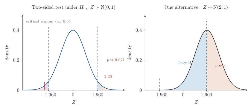
Definition 5 (Neyman–Pearson approach) Fix a significance level \alpha. Among critical regions whose type I error is at most \alpha, choose one whose type II error is as small as possible.
For the serves, C=\{c,\ldots,15\}, and the type I error is \mathbb{P}_{H_0}(X\ge c). Under \operatorname{Bin}(15,0.6), \mathbb{P}(X\ge12)=0.0905 and \mathbb{P}(X\ge13)=0.0271. At \alpha=0.05 the largest allowed region is \{13,14,15\}, and the actual size of the test is 0.0271, not 0.05. A discrete statistic usually cannot hit \alpha exactly.
Definition 6 (Power function) For a test with critical region C, the power at \theta is \operatorname{Power}(\theta)=\mathbb{P}_\theta(T\in C). On \Theta_1 it equals one minus the type II error at \theta, and on \Theta_0 it is the type I error. Its graph is the power curve.
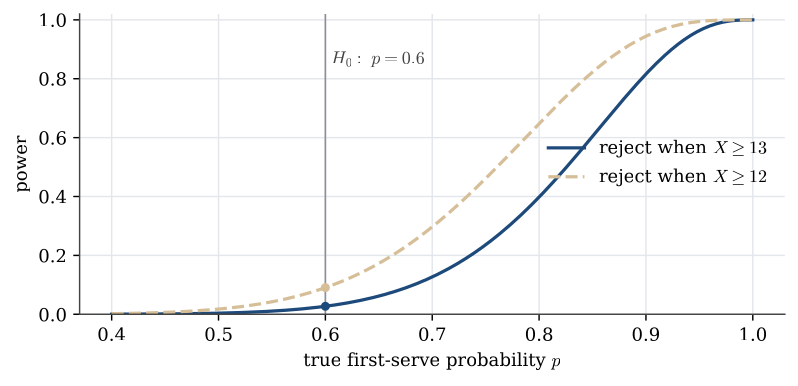
One test is better than another at the same size if its power curve lies above the other’s on the whole alternative. With 15 serves, no test of size 0.05 has much power against a moderate improvement. That is a statement about the sample size, not about the player.
The two decision rules agree. Rejecting when T falls in the level-\alpha critical region is the same as rejecting when the p-value is at most \alpha. The p-value is the smallest significance level at which this sample would reject H_0. Reporting the p-value says more than reporting a decision at a level chosen in advance.
The eight steps
A test written out in full has eight steps.
- State a statistical model for the data.
- State the null and alternative hypotheses, in terms of the model’s parameters.
- Choose the test statistic.
- Give its distribution under H_0.
- Compute its observed value.
- Compute the p-value, or the critical region for a chosen \alpha.
- Accept or reject H_0.
- State the conclusion in the language of the original question.
Example 1 (A gene in lake fish) A gene occurs in 15% of a fish population. In a sample of 100 fish from one lake, 10 carry it.
Question. Is there evidence that the lake population differs?
Solution. (1) Let X be the number of carriers among 100, X\sim\operatorname{Bin}(100,p). (2) H_0:p=0.15 against H_1:p\neq0.15; the alternative is the claim that the lake is different. (3) The statistic is X. (4) Under H_0, X\sim\operatorname{Bin}(100,0.15). (5) x=10. (6) The two-sided p-value is 2\mathbb{P}_{H_0}(X\le10)=2\times0.0994=0.199. The normal approximation \operatorname{N}(15,12.75) gives 2\Phi\{(10-15)/\sqrt{12.75}\}=2\Phi(-1.40)=0.161, and with the continuity correction, 2\Phi\{(10.5-15)/\sqrt{12.75}\}=0.208, close to the exact value. (7) The p-value is large, so H_0 is not rejected. (8) There is no evidence that the proportion of carriers in the lake differs from 15%.
Tests for a normal mean and variance
The one-sample t test
Let X_1,\ldots,X_n be independent \operatorname{N}(\mu,\sigma^2) with both parameters unknown, and test H_0:\mu=\mu_0. The statistic \overline X alone will not do. The null hypothesis really says \mu=\mu_0 with \sigma^2 anything, and the null distribution of \overline X depends on that unknown \sigma^2. A deviation of 0.5 is huge if \sigma is tiny and negligible if \sigma is large. Measuring the deviation in units of the estimated standard error fixes this.
Definition 7 (One-sample t test) For a normal random sample, the one-sample t statistic for H_0:\mu=\mu_0 is
T=\frac{\overline X-\mu_0}{s/\sqrt n},
which has the t_{n-1} distribution under H_0, whatever the value of \sigma^2. At level \alpha, reject when T\ge t_{n-1;1-\alpha} against \mu>\mu_0, when T\le-t_{n-1;1-\alpha} against \mu<\mu_0, and when |T|\ge t_{n-1;1-\alpha/2} against \mu\neq\mu_0.
The two-sided test is a left and a right one-sided test, each at level \alpha/2. If \sigma is known, the same roles are played by Z=(\overline X-\mu_0)/(\sigma/\sqrt n), which is standard normal under H_0, with the normal quantiles z_{1-\alpha} and z_{1-\alpha/2} in place of the t quantiles. That is the z test. The critical value for a two-sided z test of size 0.05 is 1.96.
Example 2 (Caffeine in cola) A claim is that regular cola contains 19 mg of caffeine per serving. For n=40 servings of another brand, \overline x=19.57 mg and s=1.40 mg.
Question. At level 0.01, is the mean caffeine content of this brand more than 19 mg?
Solution. Model the servings as a normal random sample. Test H_0:\mu=19 against H_1:\mu>19. The statistic is
t=\frac{19.57-19}{1.40/\sqrt{40}}=2.575,
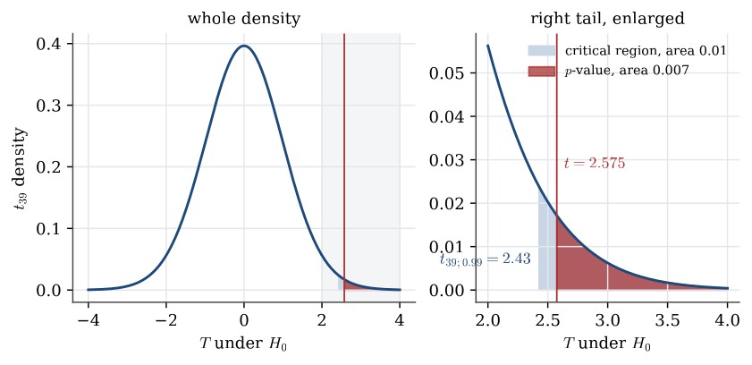
against t_{39}. The critical value is t_{39;0.99}=2.43, so t is in the critical region, and the p-value is 0.007. Reject H_0: there is strong evidence that the mean exceeds 19 mg.
Statistical significance is not practical significance. The one-sided 99% lower confidence bound is 19.57-2.43\times1.40/\sqrt{40}=19.03, so the data are consistent with a mean barely above 19. The two-sided 99% interval, (18.97,\ 20.17), even includes 19, because it spends only half its error on each side. Whether a mean of 19.5 or 20 mg matters for health is a question the test cannot answer.
The chi-squared test for a variance
For the variance, (n-1)s^2/\sigma_0^2 is \chi^2_{n-1} when \sigma^2=\sigma_0^2. Reject for large values against \sigma^2>\sigma_0^2, using \chi^2_{n-1;1-\alpha}; for small values against \sigma^2<\sigma_0^2, using \chi^2_{n-1;\alpha}; and in either tail, at \alpha/2 each, against \sigma^2\neq\sigma_0^2.
Example 3 (Tuning-fork variability) Tuning-fork frequencies have been \operatorname{N}(\mu,1.1). A new process is meant to reduce the variance. A batch of 7 new forks has sample variance 0.488.
Question. Is there evidence that the new process has smaller variance?
Solution. Test H_0:\sigma^2=1.1 against H_1:\sigma^2<1.1 with 6s^2/1.1, which is \chi^2_6 under H_0. Its value is 6\times0.488/1.1=2.66, and the p-value is \mathbb{P}(\chi^2_6\le2.66)=0.15. At level 0.05 the critical region is (0,\ 1.635], and 2.66 is not in it. There is not enough evidence that the new process is less variable. With only 7 forks, the sample variance would have to be below 0.30 to reject.
Two samples
A student believes third-year students weigh more than first-year students. A sample of 15 first-years has mean 62.0 kg and standard deviation 15 kg; a sample of 10 third-years has mean 71.5 kg and standard deviation 12 kg. Model the two groups as independent normal samples, \operatorname{N}(\mu_1,\sigma_1^2) for first-years and \operatorname{N}(\mu_2,\sigma_2^2) for third-years.
Definition 8 (Two-sample t test) For two independent normal samples with a common variance, the two-sample t statistic for H_0:\mu_1-\mu_2=\delta_0 is
T=\frac{\overline X_1-\overline X_2-\delta_0}{s_p\sqrt{1/n_1+1/n_2}},
with s_p^2 the pooled variance. Under H_0, T has the t_{n_1+n_2-2} distribution. The rejection regions are those of the one-sample test with n_1+n_2-2 degrees of freedom.
For the weights, H_0:\mu_1=\mu_2 against H_1:\mu_1<\mu_2. The pooled variance is s_p^2=(14\times15^2+9\times12^2)/23=193.3, and
t=\frac{62.0-71.5}{\sqrt{193.3\,(1/15+1/10)}}=-1.674,
on 23 degrees of freedom. Since t_{23;0.90}=1.319 and t_{23;0.95}=1.714, the p-value \mathbb{P}(T\le-1.674) lies between 0.05 and 0.10; it is 0.054. That is suggestive evidence for the student’s theory, not strong evidence. If the common \sigma were known, the same statistic with \sigma in place of s_p would be standard normal under H_0.
Definition 9 (F test for equal variances) For two independent normal samples, F=s_1^2/s_2^2 has the F_{n_1-1,n_2-1} distribution when \sigma_1^2=\sigma_2^2. Against \sigma_1^2\neq\sigma_2^2 at level \alpha, reject when F\ge F_{n_1-1,n_2-1;1-\alpha/2} or F\le1/F_{n_2-1,n_1-1;1-\alpha/2}.
The pooled t test assumes equal variances, so that assumption should be checked. For the weights, F=15^2/12^2=1.56 on (14,9) degrees of freedom. The 5% critical region is [0,\ 0.312]\cup[3.80,\ \infty), using F_{14,9;0.975}=3.80 and F_{14,9;0.025}=1/F_{9,14;0.975}=0.312. The observed value is not in it, so pooling is reasonable.
Paired samples
Did the weighing above show that a student’s weight increases between first and third year? It did not, because different students were weighed. A better design weighs the same ten students twice.
| Student | 1 | 2 | 3 | 4 | 5 | 6 | 7 | 8 | 9 | 10 |
|---|---|---|---|---|---|---|---|---|---|---|
| First year | 71.6 | 69.7 | 50.0 | 56.9 | 60.9 | 77.5 | 53.9 | 49.6 | 32.3 | 61.3 |
| Third year | 83.4 | 77.7 | 57.9 | 67.0 | 69.2 | 87.4 | 63.7 | 59.0 | 39.7 | 71.1 |
| Difference | 11.8 | 8.0 | 7.9 | 10.1 | 8.3 | 9.9 | 9.8 | 9.4 | 7.4 | 9.8 |
The two columns are not independent samples: a heavy first-year is a heavy third-year. A two-sample t test would be wrong. Instead, let D_i be the difference for student i, and model D_1,\ldots,D_{10} as a normal random sample with mean \mu_D. Testing H_0:\mu_D=0 against \mu_D>0 is a one-sample t test on the differences.
The differences have mean 9.24 and standard deviation 1.33, so t=9.24/(1.33/\sqrt{10})=21.9 on 9 degrees of freedom, with p-value about 2\times10^{-9}. The evidence that weight increases is overwhelming. Treating the columns as independent samples gives t=1.54 instead, because the large spread between students swamps the small, consistent change within each one. Pairing is the right analysis when the two measurements share a unit, a subject or a block. The dependence it removes is a covariance: \operatorname{Var}(X-Y)=\operatorname{Var} X+\operatorname{Var} Y-2\operatorname{Cov}(X,Y).
Binomial tests
One proportion
Ten people taste two yoghurts, one with an old sweetener and one with a new. Eight prefer the new one. Model the number preferring the new yoghurt as X\sim\operatorname{Bin}(10,p), and test H_0:p=0.5 against H_1:p>0.5.
Definition 10 (Binomial test) For X\sim\operatorname{Bin}(n,p) and H_0:p=p_0, the test statistic is X, with null distribution \operatorname{Bin}(n,p_0). At level \alpha, against p>p_0 reject when X\ge c, with c the smallest integer such that \mathbb{P}_{H_0}(X\ge c)\le\alpha. Against p<p_0 reject when X\le c, with c the largest integer such that \mathbb{P}_{H_0}(X\le c)\le\alpha. Against p\neq p_0, use both tails at \alpha/2 each.
Under H_0, \mathbb{P}(X\ge8)=0.055 and \mathbb{P}(X\ge9)=0.011. At level 0.05 the critical region is \{9,10\}, and x=8 is not in it, so H_0 is not rejected. The p-value is 0.055, which leaves real doubt about H_0. That a p-value of 0.055 and one of 0.045 lead to opposite decisions is a good reason to report the p-value rather than only the decision.
For large n,
Z=\frac{X-np_0}{\sqrt{np_0(1-p_0)}}
is approximately standard normal under H_0, and the normal critical values apply. The null standard error uses p_0, not \widehat p: the test asks how variable X would be if H_0 were true.
Two proportions
Of 70 viewers of a public broadcaster’s news, 40 describe themselves as left-wing; of 100 viewers of a commercial channel, 50 do. Is the public broadcaster’s audience more left-wing? Let X_1\sim\operatorname{Bin}(70,p_1) and X_2\sim\operatorname{Bin}(100,p_2) be independent, and test H_0:p_1=p_2 against H_1:p_1>p_2.
By the central limit theorem, \widehat p_1-\widehat p_2 is approximately normal with mean p_1-p_2 and variance p_1(1-p_1)/n_1+p_2(1-p_2)/n_2. Under H_0 the two proportions are a single unknown p, and the two samples together are \operatorname{Bin}(n_1+n_2,p). The maximum likelihood estimate of that common p is the pooled proportion.
Definition 11 (Two-proportion z test) For independent X_1\sim\operatorname{Bin}(n_1,p_1) and X_2\sim\operatorname{Bin}(n_2,p_2), let \widehat p=(X_1+X_2)/(n_1+n_2). The statistic for H_0:p_1=p_2 is
Z=\frac{\widehat p_1-\widehat p_2}{\sqrt{\widehat p(1-\widehat p)\,(1/n_1+1/n_2)}},
approximately standard normal under H_0 for large samples.
Here \widehat p_1=40/70=0.571, \widehat p_2=0.500 and \widehat p=90/170=0.529, so
z=\frac{0.571-0.500}{\sqrt{0.529\times0.471\times(1/70+1/100)}}=0.918,
with one-sided p-value 0.18. There is no evidence for the politician’s claim. The pooled standard error belongs to the test. The confidence interval for p_1-p_2 in Confidence intervals uses unpooled variances, because it does not assume p_1=p_2.
The sign test
All tests above assume a family of distributions up to a few parameters. A nonparametric test assumes much less.
Definition 12 (Sign test) For independent pairs (X_i,Y_i), i=1,\ldots,n, let N be the number of pairs with Y_i>X_i, ties discarded. If H_0:\mathbb{P}(Y_i>X_i)=1/2 holds, N\sim\operatorname{Bin}(n,1/2), and H_0 is tested with the binomial test.
Two examiners each mark the same 12 exams.
| Exam | 1 | 2 | 3 | 4 | 5 | 6 | 7 | 8 | 9 | 10 | 11 | 12 |
|---|---|---|---|---|---|---|---|---|---|---|---|---|
| Examiner 1 | 3.5 | 5 | 8 | 6 | 7 | 6 | 5 | 7 | 5.5 | 6.5 | 7 | 8 |
| Examiner 2 | 4 | 4.5 | 9 | 6.5 | 6.5 | 5.5 | 5.5 | 8 | 6.5 | 6 | 8 | 9 |
Examiner 2 gives the higher mark on N=8 of the 12 exams, with no ties. Against the two-sided alternative that one examiner is stricter, the p-value is 2\mathbb{P}(N\ge8)=2\times0.194=0.39, so there is no evidence of a difference. The test needs no normal model for the marks, only independent exams. The price is power: it uses only the signs of the differences, not their sizes.
Tests and intervals
A two-sided test at level \alpha and a confidence interval with confidence 1-\alpha built from the same pivot carry the same information. H_0:\theta=\theta_0 is rejected exactly when \theta_0 lies outside the interval. For the one-sample t test,
\Bigl|\frac{\overline x-\mu_0}{s/\sqrt n}\Bigr|<t_{n-1;1-\alpha/2} \iff \mu_0\in\overline x\pm t_{n-1;1-\alpha/2}\,\frac{s}{\sqrt n}.
A one-sided test pairs with a one-sided bound, as in the caffeine example. The interval is usually the more useful report. It shows which parameter values are compatible with the data, and therefore whether a significant effect is large enough to matter.
Compute how often the test statistic would look this extreme if the null hypothesis were true. That probability is the p-value. It is not the probability that the null hypothesis is true, and a small one does not say the effect is large.
Questions on this topic
Open a question to attempt it. Its worked answer is folded away at the bottom of the page.
What links here
Pages (8)
- Statistical inference — via hypothesis test
- Chi-squared tests — via two-proportion z statistic
- Analysis of variance — via Hypothesis tests
- Studies, data, and evidence — via Hypothesis tests, two-sample t test
- Using R — via Hypothesis tests
- Testing examples — via null hypothesis, Hypothesis tests, binomial test, two-sample t test
- Chi-squared examples — via null hypothesis, two-proportion z statistic
- Bayesian hypotheses and model comparison — via hypothesis test
Questions and answers (5)
See also
- Articles from this chapter: Null and alternative hypotheses · Critical region · p-value · Type I and type II errors · Neyman–Pearson approach · Power function · One-sample t test · Two-sample t test · F test for equal variances · Binomial test · Two-proportion z test · Sign test
- All statistical inference chapters
- Glossary and index
- Distribution sheet and formula lookup