Power function

Definition taught in Hypothesis tests, part of Statistical inference

Power function

Power curves for two tests of H_0:p=0.6 against p>0.6 from 15 serves. *From Hypothesis tests.*

Type	Definition
Taught in	Hypothesis tests
Part	Statistical inference
Worked examples	3

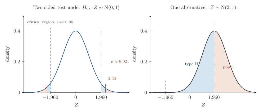
For a test with critical region C, the power at \theta is \operatorname{Power}(\theta)=\mathbb{P}_\theta(T\in C). On \Theta_1 it equals one minus the type II error at \theta, and on \Theta_0 it is the type I error. Its graph is the power curve.

Examples

Simulating the power of a t test

Worked example from Testing examples

A one-sample t test of H_0:\mu=0 against H_1:\mu>0 is run at level 0.05 on n observations.

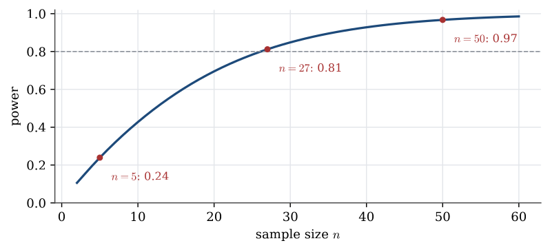
Question. What is its power if the data are really \operatorname{N}(1,2^2), with n=5 and with n=50?

Solution.

R <- 1e5; n <- 5; mu <- 1; sigma <- 2
pval <- replicate(R, {
  x <- rnorm(n, mean = mu, sd = sigma)
  1 - pt(mean(x) / (sd(x) / sqrt(n)), df = n - 1)
})
mean(pval < 0.05)                      # about 0.24
power.t.test(n = 5, delta = 1, sd = 2, sig.level = 0.05,
             type = "one.sample", alternative = "one.sided")$power   # 0.239

With five observations the test detects a mean of 1 only 24% of the time. With n=50 the power is 0.967. The power depends on \mu and \sigma only through their ratio \mu/\sigma, here 1/2, together with n and the level. A power calculation of this kind, using a guess at \sigma from a pilot study, is how a sample size is chosen before the data are collected.

Power of a serve test

Question page: Power of a serve test

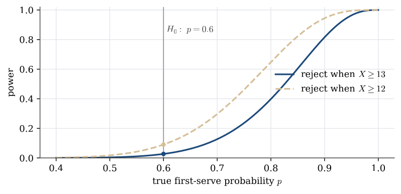
A player’s first-serve successes are modelled as X\sim\operatorname{Bin}(15,p). The test of H_0:p=0.6 against H_1:p>0.6 rejects when X\in\{13,14,15\}.

Compute the size of the test, that is the power at p=0.6.
Write the power as a function of p, and evaluate it at p=0.9.

Worked answer (click to show)

Under H_0, X\sim\operatorname{Bin}(15,0.6) and

\mathbb{P}(X\ge 13)=\sum_{k=13}^{15}\binom{15}{k}(0.6)^k(0.4)^{15-k}\approx 0.0271.

That is the size of the test. At a general p,

\mathrm{Power}(p)=\sum_{k=13}^{15}\binom{15}{k}p^k(1-p)^{15-k}.

At p=0.9 the power is about 0.816. At p=0.8 it is only 0.398: with 15 serves, a real improvement from 60% to 80% would be missed more often than not.

How small a variance?

Question page: How small a variance?

In the tuning-fork example, 7 forks are tested, H_0:\sigma^2=1.1 and H_1:\sigma^2<1.1, at level 0.05. Using \chi^2_{6;0.05}=1.635, find the largest sample variance that leads to rejection. What is the power of this test if the true variance is 0.3?

Worked answer (click to show)

The test rejects when 6s^2/1.1\le1.635, that is when s^2\le1.635\times1.1/6=0.300.

If the true variance is 0.3, then 6s^2/0.3\sim\chi^2_6, and the power is

\mathbb{P}(s^2\le0.300)=\mathbb{P}\Bigl(\frac{6s^2}{0.3}\le\frac{6\times0.300}{0.3}\Bigr)=\mathbb{P}(\chi^2_6\le5.995)\approx0.58.

Even a reduction of the variance to less than a third of its old value is detected only a little more than half the time with 7 forks.

Figures

Left: a two-sided z test of size 0.05. Under H_0 the statistic is \operatorname{N}(0,1), the critical region is the two tails beyond \pm1.960, and an observed z=2.30 has p-value 0.021. Right: under the alternative Z\sim\operatorname{N}(2,1) the same cutoffs split the density into the power, the part beyond them, and the type II error, the part between. *From Hypothesis tests.*

The power of the one-sided one-sample t test at level 0.05 against a true mean of half a standard deviation, as the sample size grows. It passes 0.8 at about n=27. *From Testing examples.*

Used in

Taught in Hypothesis tests, where the derivation and examples are.
All 6 questions on Hypothesis tests