One-sample t test

Definition taught in Hypothesis tests, part of Statistical inference

One-sample t test

The caffeine test below. *From Hypothesis tests.*

Type	Definition
Taught in	Hypothesis tests
Part	Statistical inference
Properties	1
Worked examples	4

For a normal random sample, the one-sample t statistic for H_0:\mu=\mu_0 is

T=\frac{\overline X-\mu_0}{s/\sqrt n},

which has the t_{n-1} distribution under H_0, whatever the value of \sigma^2. At level \alpha, reject when T\ge t_{n-1;1-\alpha} against \mu>\mu_0, when T\le-t_{n-1;1-\alpha} against \mu<\mu_0, and when |T|\ge t_{n-1;1-\alpha/2} against \mu\neq\mu_0.

Properties

One-sample t pivot

Main article: One-sample t pivot

If X_1,\ldots,X_n are independent and \operatorname{N}(\mu,\sigma^2), then

T=\frac{\overline X-\mu}{s/\sqrt n}

has a Student t distribution with n-1 degrees of freedom. A Student variable with m degrees of freedom is Z/\sqrt{V/m} where Z is standard normal, V is chi-squared with m degrees of freedom, and Z and V are independent.

Examples

Caffeine in cola

Worked example from Hypothesis tests

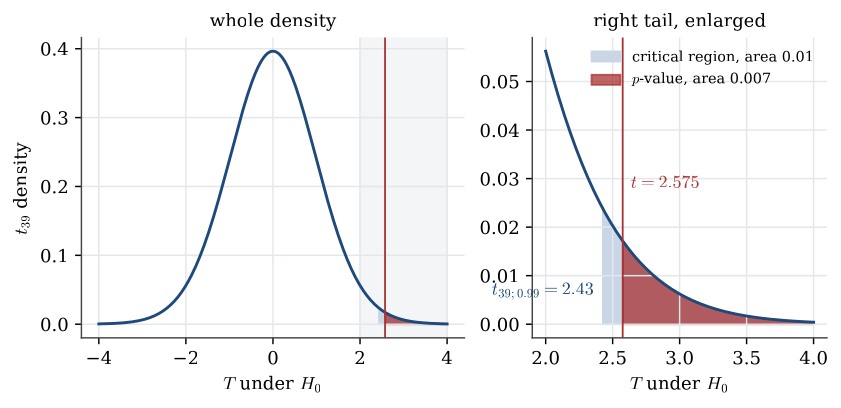
A claim is that regular cola contains 19 mg of caffeine per serving. For n=40 servings of another brand, \overline x=19.57 mg and s=1.40 mg.

Question. At level 0.01, is the mean caffeine content of this brand more than 19 mg?

Solution. Model the servings as a normal random sample. Test H_0:\mu=19 against H_1:\mu>19. The statistic is

t=\frac{19.57-19}{1.40/\sqrt{40}}=2.575,

against t_{39}. The critical value is t_{39;0.99}=2.43, so t is in the critical region, and the p-value is 0.007. Reject H_0: there is strong evidence that the mean exceeds 19 mg.

Statistical significance is not practical significance. The one-sided 99% lower confidence bound is 19.57-2.43\times1.40/\sqrt{40}=19.03, so the data are consistent with a mean barely above 19. The two-sided 99% interval, (18.97,\ 20.17), even includes 19, because it spends only half its error on each side. Whether a mean of 19.5 or 20 mg matters for health is a question the test cannot answer.

Simulating the power of a t test

Worked example from Testing examples

A one-sample t test of H_0:\mu=0 against H_1:\mu>0 is run at level 0.05 on n observations.

Question. What is its power if the data are really \operatorname{N}(1,2^2), with n=5 and with n=50?

Solution.

R <- 1e5; n <- 5; mu <- 1; sigma <- 2
pval <- replicate(R, {
  x <- rnorm(n, mean = mu, sd = sigma)
  1 - pt(mean(x) / (sd(x) / sqrt(n)), df = n - 1)
})
mean(pval < 0.05)                      # about 0.24
power.t.test(n = 5, delta = 1, sd = 2, sig.level = 0.05,
             type = "one.sample", alternative = "one.sided")$power   # 0.239

With five observations the test detects a mean of 1 only 24% of the time. With n=50 the power is 0.967. The power depends on \mu and \sigma only through their ratio \mu/\sigma, here 1/2, together with n and the level. A power calculation of this kind, using a guess at \sigma from a pilot study, is how a sample size is chosen before the data are collected.

Two labs on the same patients

Worked example from Testing examples

Two labs measure the same quantity on the same 15 patients.

lab1 <- c(22, 18, 28, 26, 13, 8, 21, 26, 27, 29, 25, 24, 22, 28, 15)
lab2 <- c(25, 21, 31, 27, 11, 10, 25, 26, 29, 28, 26, 23, 22, 25, 17)

Question. Do the labs differ on average?

Solution. The two columns are not independent: a patient with a low value gets it from both labs, as patient 6 does with 8 and 10. So analyse the differences D_i=X_i-Y_i as one sample, D_i\sim\operatorname{N}(\delta,\sigma^2), and test H_0:\delta=0 against \delta\neq0:

t.test(lab1, lab2, paired = TRUE)
# t = -1.7618, df = 14, p-value = 0.0999

The mean difference is -0.93 with standard deviation 2.05, so t=-0.93/(2.05/\sqrt{15})=-1.76 and p=0.10. There is weak evidence, at most, that lab 2 reads higher. Ignoring the pairing and running a two-sample test gives t=-0.42 and p=0.68: the large differences between patients swamp the small, consistent difference between labs. Pairing removes the patient effect.

Tyre wear on five cars

Question page: Tyre wear on five cars

Each of five cars carries one tyre of type A and one of type B. Tread thickness after 10000 km is

Car	1	2	3	4	5
Type A	10.6	9.8	12.3	9.7	8.8
Type B	10.2	9.4	11.8	9.1	8.3

Test whether the mean tread differs between the two types, at level 0.05. Use t_{4;0.975}=2.776.

Worked answer (click to show)

The differences A minus B are 0.4, 0.4, 0.5, 0.6 and 0.5, with mean \overline d=0.48 and standard deviation s_d=0.0837. Model them as a normal random sample with mean \mu_D, and test H_0:\mu_D=0 against \mu_D\neq0:

t=\frac{0.48}{0.0837/\sqrt5}=\frac{0.48}{0.0374}=12.8.

Since 12.8>t_{4;0.975}=2.776, reject H_0; the two-sided p-value is 0.0002. Type A keeps more tread. Ignoring the pairing and comparing the two columns as independent samples would be wrong: the variation between cars, from 8.3 to 12.3, is far larger than the difference between tyres.

Used in

Taught in Hypothesis tests, where the derivation and examples are.
All 6 questions on Hypothesis tests