One-sample t pivot
Theorem taught in Confidence intervals, part of Statistical inference
One-sample t pivot
| Type | Theorem |
| Taught in | Confidence intervals |
| Part | Statistical inference |
| Worked examples | 3 |
If X_1,\ldots,X_n are independent and \operatorname{N}(\mu,\sigma^2), then
T=\frac{\overline X-\mu}{s/\sqrt n}
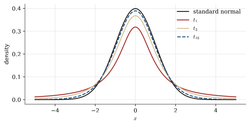
has a Student t distribution with n-1 degrees of freedom. A Student variable with m degrees of freedom is Z/\sqrt{V/m} where Z is standard normal, V is chi-squared with m degrees of freedom, and Z and V are independent.
Examples
Household fuel spending
Worked example from Confidence intervals
An oil company samples 51 households at random from a city. They spent on average \overline x=1136 dollars a year on petrol and heating oil, with bias-corrected standard deviation s=178 dollars.
Question. Give a 95% confidence interval for the mean spending \mu in the city, and say what the model assumes.
Solution. Model the spending of the 51 households as a random sample from \operatorname{N}(\mu,\sigma^2), both unknown. Random selection justifies independence and a common distribution. Normality is an assumption; with n=51 the central limit theorem makes it matter little for an interval about the mean. With t_{50;0.975}=2.009, the standard error is 178/\sqrt{51}=24.93, and
1136\pm2.009\times24.93=1136\pm50.1=(1085.9,\ 1186.1).
Ten normal measurements
Worked example from Estimation examples
Ten measurements, modelled as a \operatorname{N}(\mu,\sigma^2) sample, are
77.01,\ 71.37,\ 77.15,\ 79.89,\ 76.46,\ 78.10,\ 77.18,\ 74.08,\ 75.88,\ 72.63.
Question. Estimate \mu and \sigma, and give a 95% interval for \mu.
Solution.
x <- c(77.01, 71.37, 77.15, 79.89, 76.46, 78.10, 77.18, 74.08, 75.88, 72.63)
mean(x); sd(x)              # 75.975  2.581
t.test(x)$conf.int          # 74.13  77.82
The estimates are \widehat\mu=\overline x=75.975 and s=2.58. The t interval uses t_{9;0.975}=2.262: 75.975\pm2.262\times2.58/\sqrt{10}=(74.13,\ 77.82). With only ten values the t quantile matters; the normal quantile 1.96 would give an interval about 13% too short.
The volume of a drop
Worked example from Estimation examples
A burette reads 25.36 mL, then 22.84 mL after 50 drops, then 20.36 mL after another 50.
Question. Give a 95% interval for the volume of one drop.
Solution. The two batches of 50 drops have volumes x_1=2.52 and x_2=2.48 mL. Model them as a \operatorname{N}(\mu,\sigma^2) sample of size n=2, where \mu is the expected volume of 50 drops. Then \overline x=2.50, s=0.02\sqrt2, and the standard error is s/\sqrt2=0.02. With one degree of freedom t_{1;0.975}=12.71, so the interval for \mu is
2.50\pm12.71\times0.02=(2.25,\ 2.75).
Dividing by 50, a monotone change of scale, gives a 95% interval for one drop of (0.045,\ 0.055) mL. The huge quantile 12.71 is the price of estimating a standard deviation from two numbers.
Used in
- Taught in Confidence intervals, where the derivation and examples are.
- All 6 questions on Confidence intervals
See also
Confidence interval · Pivot · Pooled variance · Two-sample t pivot · Variance-ratio F pivot · Wald interval