Bayesian hypotheses and model comparison
Part of Bayesian statistics · 15 questions on this topic · What links here
Bayesian hypotheses and model comparison
| Part | Bayesian statistics |
| Chapter | 6 of 9 in this part |
| Previous | Categorical data and the Dirichlet distribution |
| Next | Exponential families and conjugacy |
| Questions | 15 |
| Definitions | Posterior hypothesis probability · Marginal likelihood and Bayes factor |
| Results | Bayes action for two hypotheses · Posterior-odds factorisation |
| Figures | 1 |
Probability statements and decisions
Definition 1 (Posterior hypothesis probability) Suppose a parameter space \Omega is partitioned into regions \Omega_0 and \Omega_1. A test that instead reports a long-run p-value under a null sampling model is a hypothesis test. Numerical examples of those tests are in Testing examples. The posterior hypothesis probabilities are \begin{align*} \mathbb{P}(H_0\mid x) &=\mathbb{P}(\theta\in\Omega_0\mid x) =\int_{\Omega_0}p(\theta\mid x)\,\mathrm{d}\theta,\\ \mathbb{P}(H_1\mid x) &=\mathbb{P}(\theta\in\Omega_1\mid x) =\int_{\Omega_1}p(\theta\mid x)\,\mathrm{d}\theta. \end{align*} If the two regions exhaust the support, the probabilities sum to one.
Proposition 1 (Bayes action for two hypotheses) These probabilities do not by themselves define an action. If choosing action a_0 when H_1 is true costs L_{01} and choosing a_1 when H_0 is true costs L_{10}, the posterior expected losses are
\rho(a_0\mid x)=L_{01}\mathbb{P}(H_1\mid x), \qquad \rho(a_1\mid x)=L_{10}\mathbb{P}(H_0\mid x).
Choose a_0 when \begin{align*} L_{01}\mathbb{P}(H_1\mid x) &<L_{10}\mathbb{P}(H_0\mid x)\\ \Longleftrightarrow\quad \frac{\mathbb{P}(H_0\mid x)}{\mathbb{P}(H_1\mid x)} &>\frac{L_{01}}{L_{10}}. \end{align*} Equal losses reduce the threshold to one. This separates the probability calculation from the decision rule.
The Bayesian calculation need not force an all-or-nothing verdict. A useful practice is to report the posterior support for each hypothesis and to let the action depend on the real consequences of being wrong. If a decision is compulsory, losses provide the threshold. Reporting evidence and choosing an action are related tasks, but they are not the same task. This is also why Bayesians are often less enthusiastic about compulsory model selection than about reporting posterior model probabilities.1
In frequentist design, type-I and type-II error rates \alpha and \beta are properties of repeated use of a test. Values such as 0.05 and 0.20 are planning choices, not scientific constants, and sample-size calculations also require an effect size worth detecting.
Poisson imperfect-fruit example
Example 1 (Imperfect-fruit decision) Let X_i be the number of imperfect pieces in box i, with about 100 pieces per box. “Imperfect” must be defined before the data are collected so that producer and analyst classify fruit in the same way. The model is
X_i\mid\theta\stackrel{\mathrm{iid}}{\sim}\operatorname{Poisson}(\theta), \qquad H_0:\theta\leq10, \quad H_1:\theta>10.
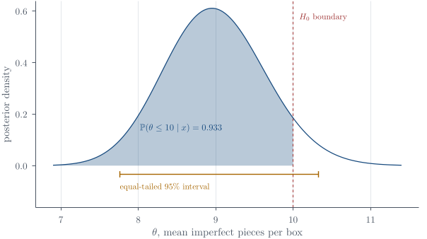
For the observed sample, n=20 and S=\sum_i x_i=177; the stated prior is \theta\sim\operatorname{Gamma}(12,1) in shape–rate form.
Question. Find the posterior distribution, the posterior probabilities and odds for H_0 and H_1, and an equal-tailed 95\% credible interval. Explain why the interval may cross 10 even when most posterior mass lies below it.
Solution. Because the posterior for \theta is continuous,
\mathbb{P}(\theta=10\mid{\boldsymbol{x}})=0.
Consequently it makes no numerical difference whether equality is assigned to H_0 or H_1. This is a statement about the continuous parameter, even though the observed fruit counts are discrete.
For n boxes and S=\sum_i x_i, the likelihood is \begin{aligned} p({\boldsymbol{x}}\mid\theta) &=\prod_{i=1}^n\frac{e^{-\theta}\theta^{x_i}}{x_i!}\\ &=\left(\prod_{i=1}^n\frac1{x_i!}\right) e^{-n\theta}\theta^{\sum_i x_i}\\ &\propto e^{-n\theta}\theta^S. \end{aligned} \qquad(1) The working total is S=177 for n=20.
The stated prior is \theta\sim\operatorname{Gamma}(12,1) in the standard shape–rate convention, so
p(\theta)=\frac1{\Gamma(12)}\theta^{12-1}e^{-\theta} \propto\theta^{11}e^{-\theta}.
Multiplying by the likelihood gives \begin{align*} p(\theta\mid{\boldsymbol{x}}) &\propto \theta^S e^{-n\theta}\theta^{11}e^{-\theta}\\ &=\theta^{S+11}e^{-(n+1)\theta}\\ &=\theta^{189-1}e^{-21\theta}. \end{align*} Therefore the internally consistent shape–rate update is \boxed{\theta\mid{\boldsymbol{x}}\sim\operatorname{Gamma}(189,21)}. \qquad(2) Its posterior mean is
\mathbb{E}(\theta\mid{\boldsymbol{x}})=\frac{189}{21}=9.
The MLE is S/n=177/20=8.85. Although the prior mean 12 lies above the boundary 10, the data move the posterior centre below it.
Let \gamma(a,z)=\int_0^zt^{a-1}e^{-t}\,\mathrm{d} t be the lower incomplete Gamma function. If T\sim\operatorname{Gamma}(a,b), then
\mathbb{P}(T\leq t)=\frac{\gamma(a,bt)}{\Gamma(a)}.
Consequently, \begin{align*} \mathbb{P}(H_0\mid{\boldsymbol{x}}) &=\mathbb{P}(\theta\leq10\mid{\boldsymbol{x}})\\ &=\frac{\gamma(189,21\cdot10)}{\Gamma(189)}\\ &=0.93298381,\\ \mathbb{P}(H_1\mid{\boldsymbol{x}})&=1-0.93298381=0.06701619. \end{align*} The posterior odds are
\frac{\mathbb{P}(H_0\mid{\boldsymbol{x}})}{\mathbb{P}(H_1\mid{\boldsymbol{x}})} =\frac{0.93298381}{0.06701619} \approx13.92.
The equal-tailed 95\% credible interval is approximately (7.76,10.33). It crosses 10, while 93.3\% of posterior mass lies at or below 10. These are different summaries: interval inclusion does not produce a general accept/reject rule for an interval hypothesis.
A convention check uses the other Gamma convention. Writing a prior kernel p(\theta)\propto\theta^\alpha e^{-\beta\theta} with \alpha=12 describes \operatorname{Gamma}(13,1), not the stated \operatorname{Gamma}(12,1). That alternative gives \theta\mid x\sim\operatorname{Gamma}(190,21), posterior mean 190/21\approx9.05, \mathbb{P}(\theta\leq10\mid x)=0.92320087, odds 12.02, and interval (7.81,10.38). The main calculation above follows the stated shape–rate prior; the alternative is retained here so that neither that result nor the convention error is hidden.
Posterior odds and Bayes factors
Theorem 1 (Posterior-odds factorisation) For two models M_1 and M_2, Bayes’ rule gives
\mathbb{P}(M_j\mid x) =\frac{p(x\mid M_j)\mathbb{P}(M_j)}{p(x)}.
Taking the ratio cancels the common evidence p(x): \begin{aligned} \frac{\mathbb{P}(M_1\mid x)}{\mathbb{P}(M_2\mid x)} &=\frac{p(x\mid M_1)\mathbb{P}(M_1)/p(x)} {p(x\mid M_2)\mathbb{P}(M_2)/p(x)}\\ &=\underbrace{\frac{p(x\mid M_1)}{p(x\mid M_2)}}_{ \operatorname{BF}_{12}} \underbrace{\frac{\mathbb{P}(M_1)}{\mathbb{P}(M_2)}}_{ \text{prior odds}}. \end{aligned} \qquad(3)
Definition 2 (Marginal likelihood and Bayes factor) The marginal likelihood in model M_j is p(x\mid M_j) =\int p(x\mid\theta_j,M_j) p(\theta_j\mid M_j)\,\mathrm{d}\theta_j. \qquad(4) It averages the likelihood over the parameter prior; it does not evaluate the likelihood at a fitted maximum. The Bayes factor comparing M_1 with M_2 is \operatorname{BF}_{12}=p(x\mid M_1)/p(x\mid M_2).
A Bayes factor compares whole models, not merely their best-fitting parameter values. The marginal likelihood averages over each model’s prior parameter space, so diffuse priors can spread support across many poor explanations and change the comparison. Equal prior model probabilities are a transparent modelling choice, not a mathematical requirement. Model probabilities, parameter priors, and the set of models under consideration must all be stated before a numerical ratio can be interpreted responsibly.
Remark 1 (A hypothesis region is not a separate model). Two constructions must not be confused:
If H_0 and H_1 are regions of one parameter space, compute one posterior and integrate it over the regions.
If M_1 and M_2 have different dimensions or parameterisations, each model needs its own parameter prior and marginal likelihood. A continuous prior on the larger space assigns probability zero to a lower-dimensional surface.
The fruit example is the first construction. Independence in the advertising table is the second.
Bayes factor for independence in the 2\times3 table
Let M_1 be the unrestricted six-cell multinomial and M_2 impose independence of gender and response. We assign equal model probabilities, so the prior odds are one. This is a stated modelling choice, not an automatic default.
Unrestricted model M_1
Under
{\boldsymbol{p}}\mid M_1\sim\operatorname{Dirichlet}(1,1,1,1,1,1),
the prior density is
\frac{\Gamma(6)}{\Gamma(1)^6}=120.
The fact that a uniform density equals 120 rather than 1 reflects the volume of the five-dimensional simplex.
Let C=501!/\prod_{k=1}^6x_k! be the multinomial coefficient. Then \begin{aligned} p({\boldsymbol{x}}\mid M_1) &=\int C\prod_{k=1}^6p_k^{x_k}\,120\,\mathrm{d}{\boldsymbol{p}}\\ &=120C\,B(x_1+1,\ldots,x_6+1)\\ &=120\frac{501!}{\prod_kx_k!} \frac{\prod_k\Gamma(x_k+1)}{\Gamma(501+6)}\\ &=120\frac{501!}{\prod_kx_k!} \frac{\prod_kx_k!}{\Gamma(507)}\\ &=\frac{501!\Gamma(6)}{\Gamma(507)}\\ &=\binom{506}{5}^{-1}\\ &=3.690091\times10^{-12}. \end{aligned} \qquad(5) The cell factorials cancel, so this prior predictive probability is the same for every six-cell count vector with total 501.
Independence model M_2
Write
p_{ij}=r_i c_j, \qquad r_1+r_2=1, \qquad c_1+c_2+c_3=1.
Use independent uniform priors
(r_1,r_2)\sim\operatorname{Dirichlet}(1,1), \qquad (c_1,c_2,c_3)\sim\operatorname{Dirichlet}(1,1,1).
Their joint density is
\frac{\Gamma(2)}{\Gamma(1)^2} \frac{\Gamma(3)}{\Gamma(1)^3}=1\cdot2=2.
Substituting p_{ij}=r_ic_j into the cell likelihood and grouping row and column exponents gives \begin{align*} \prod_{i=1}^2\prod_{j=1}^3p_{ij}^{x_{ij}} &=\prod_{i,j}(r_ic_j)^{x_{ij}}\\ &=\prod_i r_i^{\sum_jx_{ij}} \prod_j c_j^{\sum_ix_{ij}}\\ &=r_1^{257}r_2^{244} c_1^{146}c_2^{95}c_3^{260}. \end{align*} The marginal likelihood separates into two Dirichlet integrals: \begin{aligned} p({\boldsymbol{x}}\mid M_2) &=2C \int r_1^{257}r_2^{244}\,\mathrm{d}{\boldsymbol{r}} \int c_1^{146}c_2^{95}c_3^{260}\,\mathrm{d}{\boldsymbol{c}}\\ &=2C\,B(258,245)B(147,96,261)\\ &=9.212201\times10^{-15}. \end{aligned} \qquad(6)
The Bayes factor is therefore \begin{align*} \operatorname{BF}_{12} &=\frac{3.690091\times10^{-12}} {9.212201\times10^{-15}}\\ &=400.57. \end{align*} With equal prior odds, the posterior odds are 400.57:1, giving
\mathbb{P}(M_1\mid{\boldsymbol{x}}) =\frac{400.57}{1+400.57}\approx0.9975, \qquad \mathbb{P}(M_2\mid{\boldsymbol{x}})\approx0.0025.
Under the specified models and priors, the table is strong evidence that response depends on gender.
A frequentist likelihood-ratio or Pearson \chi^2 analysis of the same table would probably reach the same qualitative conclusion by different workings. A frequentist comparison is not carried out here, so this is calibration, not a claim that the two inferential statements or their assumptions are identical.
The departure is visible in the raw rates:
\frac{147}{257}\approx0.572, \qquad \frac{113}{244}\approx0.463.
Under independence, the expected male-negative count based on observed margins is
\frac{257\cdot146}{501}\approx74.9,
compared with 53 observed.
Bayes factors automatically average over unused parameter space, creating a complexity penalty. They are also sensitive to parameter priors because Equation 4 averages over the whole prior. A responsible model comparison therefore checks defensible alternatives such as uniform, Jeffreys, and weakly informative Dirichlet concentrations.
Questions on this topic
Open a question to attempt it. Its worked answer is folded away at the bottom of the page.
What links here
Pages (6)
- Hypothesis tests — via Bayes factor, Bayesian hypotheses and model comparison
- Using R — via Bayesian hypotheses and model comparison
- Testing examples — via Bayesian hypotheses and model comparison
- Bayesian foundations — via marginal likelihood
- How to use the final preparation — via Bayes factors
- Reference formulas and problem-solving workflow — via marginal likelihood
Questions and answers (15)
- Who owns the boundary? · Make the simplex integral equal one · Two routes to the same table · An IQ threshold · Q5 (answer) · Q11 (answer) · Q15 (answer) · Q21 · Q29 · Q44 · Q53 · Question 8 · Question 15 · Question 18 · C8
See also
- Articles from this chapter: Posterior hypothesis probability · Bayes action for two hypotheses · Posterior-odds factorisation · Marginal likelihood and Bayes factor · A hypothesis region is not a separate model
- All bayesian statistics chapters
- Glossary and index
- Distribution sheet and formula lookup
Footnotes
If an action really must be taken, the consequences belong in the loss function. A threshold smuggled in after the probability calculation is still a decision rule; it is merely a less candid one.↩︎