Posterior hypothesis probability
Definition taught in Bayesian hypotheses and model comparison, part of Bayesian statistics
Posterior hypothesis probability
| Type | Definition |
| Taught in | Bayesian hypotheses and model comparison |
| Part | Bayesian statistics |
| Properties | 2 |
| Worked examples | 3 |
| Questions using it | 5 |
Suppose a parameter space \Omega is partitioned into regions \Omega_0 and \Omega_1. A test that instead reports a long-run p-value under a null sampling model is a hypothesis test. Numerical examples of those tests are in Testing examples. The posterior hypothesis probabilities are \begin{align*} \mathbb{P}(H_0\mid x) &=\mathbb{P}(\theta\in\Omega_0\mid x) =\int_{\Omega_0}p(\theta\mid x)\,\mathrm{d}\theta,\\ \mathbb{P}(H_1\mid x) &=\mathbb{P}(\theta\in\Omega_1\mid x) =\int_{\Omega_1}p(\theta\mid x)\,\mathrm{d}\theta. \end{align*} If the two regions exhaust the support, the probabilities sum to one.
Properties
Bayes action for two hypotheses
Main article: Bayes action for two hypotheses
These probabilities do not by themselves define an action. If choosing action a_0 when H_1 is true costs L_{01} and choosing a_1 when H_0 is true costs L_{10}, the posterior expected losses are
\rho(a_0\mid x)=L_{01}\mathbb{P}(H_1\mid x), \qquad \rho(a_1\mid x)=L_{10}\mathbb{P}(H_0\mid x).
Choose a_0 when \begin{align*} L_{01}\mathbb{P}(H_1\mid x) &<L_{10}\mathbb{P}(H_0\mid x)\\ \Longleftrightarrow\quad \frac{\mathbb{P}(H_0\mid x)}{\mathbb{P}(H_1\mid x)} &>\frac{L_{01}}{L_{10}}. \end{align*} Equal losses reduce the threshold to one. This separates the probability calculation from the decision rule.
Posterior-odds factorisation
Main article: Posterior-odds factorisation
For two models M_1 and M_2, Bayes’ rule gives
\mathbb{P}(M_j\mid x) =\frac{p(x\mid M_j)\mathbb{P}(M_j)}{p(x)}.
Taking the ratio cancels the common evidence p(x): \begin{aligned} \frac{\mathbb{P}(M_1\mid x)}{\mathbb{P}(M_2\mid x)} &=\frac{p(x\mid M_1)\mathbb{P}(M_1)/p(x)} {p(x\mid M_2)\mathbb{P}(M_2)/p(x)}\\ &=\underbrace{\frac{p(x\mid M_1)}{p(x\mid M_2)}}_{ \operatorname{BF}_{12}} \underbrace{\frac{\mathbb{P}(M_1)}{\mathbb{P}(M_2)}}_{ \text{prior odds}}. \end{aligned}
Examples
Imperfect-fruit decision
Worked example from Bayesian hypotheses and model comparison
Let X_i be the number of imperfect pieces in box i, with about 100 pieces per box. “Imperfect” must be defined before the data are collected so that producer and analyst classify fruit in the same way. The model is
X_i\mid\theta\stackrel{\mathrm{iid}}{\sim}\operatorname{Poisson}(\theta), \qquad H_0:\theta\leq10, \quad H_1:\theta>10.
For the observed sample, n=20 and S=\sum_i x_i=177; the stated prior is \theta\sim\operatorname{Gamma}(12,1) in shape–rate form.
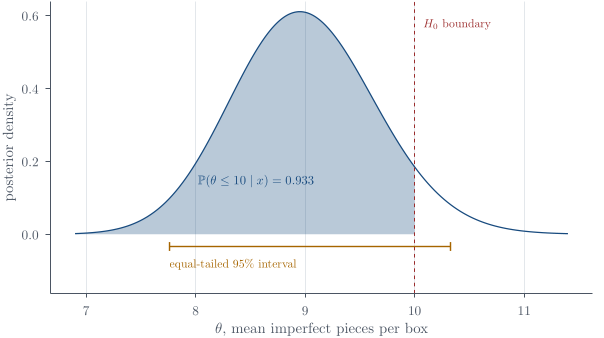
Question. Find the posterior distribution, the posterior probabilities and odds for H_0 and H_1, and an equal-tailed 95\% credible interval. Explain why the interval may cross 10 even when most posterior mass lies below it.
Solution. Because the posterior for \theta is continuous,
\mathbb{P}(\theta=10\mid{\boldsymbol{x}})=0.
Consequently it makes no numerical difference whether equality is assigned to H_0 or H_1. This is a statement about the continuous parameter, even though the observed fruit counts are discrete.
For n boxes and S=\sum_i x_i, the likelihood is \begin{aligned} p({\boldsymbol{x}}\mid\theta) &=\prod_{i=1}^n\frac{e^{-\theta}\theta^{x_i}}{x_i!}\\ &=\left(\prod_{i=1}^n\frac1{x_i!}\right) e^{-n\theta}\theta^{\sum_i x_i}\\ &\propto e^{-n\theta}\theta^S. \end{aligned} The working total is S=177 for n=20.
The stated prior is \theta\sim\operatorname{Gamma}(12,1) in the standard shape–rate convention, so
p(\theta)=\frac1{\Gamma(12)}\theta^{12-1}e^{-\theta} \propto\theta^{11}e^{-\theta}.
Multiplying by the likelihood gives \begin{align*} p(\theta\mid{\boldsymbol{x}}) &\propto \theta^S e^{-n\theta}\theta^{11}e^{-\theta}\\ &=\theta^{S+11}e^{-(n+1)\theta}\\ &=\theta^{189-1}e^{-21\theta}. \end{align*} Therefore the internally consistent shape–rate update is \boxed{\theta\mid{\boldsymbol{x}}\sim\operatorname{Gamma}(189,21)}. Its posterior mean is
\mathbb{E}(\theta\mid{\boldsymbol{x}})=\frac{189}{21}=9.
The MLE is S/n=177/20=8.85. Although the prior mean 12 lies above the boundary 10, the data move the posterior centre below it.
Let \gamma(a,z)=\int_0^zt^{a-1}e^{-t}\,\mathrm{d} t be the lower incomplete Gamma function. If T\sim\operatorname{Gamma}(a,b), then
\mathbb{P}(T\leq t)=\frac{\gamma(a,bt)}{\Gamma(a)}.
Consequently, \begin{align*} \mathbb{P}(H_0\mid{\boldsymbol{x}}) &=\mathbb{P}(\theta\leq10\mid{\boldsymbol{x}})\\ &=\frac{\gamma(189,21\cdot10)}{\Gamma(189)}\\ &=0.93298381,\\ \mathbb{P}(H_1\mid{\boldsymbol{x}})&=1-0.93298381=0.06701619. \end{align*} The posterior odds are
\frac{\mathbb{P}(H_0\mid{\boldsymbol{x}})}{\mathbb{P}(H_1\mid{\boldsymbol{x}})} =\frac{0.93298381}{0.06701619} \approx13.92.
The equal-tailed 95\% credible interval is approximately (7.76,10.33). It crosses 10, while 93.3\% of posterior mass lies at or below 10. These are different summaries: interval inclusion does not produce a general accept/reject rule for an interval hypothesis.
A convention check uses the other Gamma convention. Writing a prior kernel p(\theta)\propto\theta^\alpha e^{-\beta\theta} with \alpha=12 describes \operatorname{Gamma}(13,1), not the stated \operatorname{Gamma}(12,1). That alternative gives \theta\mid x\sim\operatorname{Gamma}(190,21), posterior mean 190/21\approx9.05, \mathbb{P}(\theta\leq10\mid x)=0.92320087, odds 12.02, and interval (7.81,10.38). The main calculation above follows the stated shape–rate prior; the alternative is retained here so that neither that result nor the convention error is hidden.
Q21. Evidence and posterior model probabilities
Question page: Q21. Evidence and posterior model probabilities
[4 marks]
An analysis produces a Bayes factor of 4 in favour of model M_1 over model M_0. Before observing the data, the researcher regarded M_0 as nine times as probable as M_1. The researcher concludes:
“The Bayes factor favours M_1, so M_1 must now have the greater posterior probability.”
Assess this conclusion. Explain how the Bayes factor changes the model odds, and identify which model has the greater posterior probability.
Definitions. The Bayes factor is B_{10}=p({\boldsymbol{x}}\mid M_1)/p({\boldsymbol{x}}\mid M_0). Odds in favour of M_1 are \mathbb P(M_1)/\mathbb P(M_0), with the analogous conditional ratio for posterior odds. The two models exhaust the comparison, so their probabilities sum to one. Here B_{10}=4 and the prior odds are 1:9.
A Bayes factor updates prior model odds according to \frac{\mathbb{P}(M_1\mid{\boldsymbol{x}})}{\mathbb{P}(M_0\mid{\boldsymbol{x}})} =B_{10} \frac{\mathbb{P}(M_1)}{\mathbb{P}(M_0)}. Because M_0 was initially nine times as probable as M_1, the prior odds in favour of M_1 are \frac{\mathbb{P}(M_1)}{\mathbb{P}(M_0)}=\frac19. With B_{10}=4, the posterior odds become \boxed{ \frac{\mathbb{P}(M_1\mid{\boldsymbol{x}})}{\mathbb{P}(M_0\mid{\boldsymbol{x}})} =4\left(\frac19\right)=\frac49. } Therefore, \mathbb{P}(M_1\mid{\boldsymbol{x}})=\frac4{13}, \qquad \mathbb{P}(M_0\mid{\boldsymbol{x}})=\frac9{13}. The data favour M_1 relative to the prior because B_{10}>1, but the evidence is not strong enough to overcome the initial nine-to-one odds in favour of M_0. Thus \boxed{ \mathbb{P}(M_0\mid{\boldsymbol{x}})> \mathbb{P}(M_1\mid{\boldsymbol{x}}). } The researcher’s conclusion is therefore incorrect: a Bayes factor favouring M_1 does not necessarily make M_1 the more probable model a posteriori.
C8. Evidence and model odds
Question page: C8. Evidence and model odds
What are marginal likelihoods and Bayes factors? How does a Bayes factor update model odds?
Definitions/notation. For model M_j with a proper parameter prior, its marginal likelihood is m_j(x)=\int p(x\mid\theta_j,M_j)p(\theta_j\mid M_j)\,d\theta_j, and BF_{12}=m_1(x)/m_2(x) is the Bayes factor for M_1 against M_2. Posterior model odds equal BF_{12} times prior model odds; the Bayes factor alone is not a posterior model probability.
Used in
- Taught in Bayesian hypotheses and model comparison, where the derivation and examples are.
- Questions that use it (5) — Who owns the boundary? · Q29 (answer) · Q44 (answer) · Question 8 (answer) · C8 (answer)
- All 15 questions on Bayesian hypotheses and model comparison
See also
Bayes action for two hypotheses · Posterior-odds factorisation · Marginal likelihood and Bayes factor · A hypothesis region is not a separate model