Beta–Binomial conjugacy
Proposition taught in The Beta–Binomial model, part of Bayesian statistics
Beta–Binomial conjugacy
| Type | Proposition |
| Taught in | The Beta–Binomial model |
| Part | Bayesian statistics |
| Worked examples | 2 |
| Questions using it | 2 |
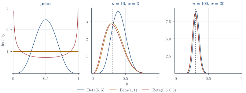
\boxed{ \theta\mid x\sim \operatorname{Beta}(\alpha+x,\beta+n-x)}.
Examples
Q6. Beta-Binomial conjugacy and prior influence
Question page: Q6. Beta-Binomial conjugacy and prior influence
Suppose X\mid\theta\sim\operatorname{Bin}(n,\theta), \qquad \theta\sim\operatorname{Beta}(a,b), where n\geq1, a,b>0, and the observed value of X is x.
(a) Derive the posterior density of \theta. Identify its distribution, parameters, and support. [3 marks]
(b) Express the posterior mean as a weighted average of the prior mean and x/n. Explain how the weight on the prior changes as n increases, with a and b fixed. [3 marks]
(c) Another statistician instead uses a prior uniform on (0,1/2). If x/n=4/5, can the posterior assign positive probability to \theta>1/2? Explain why or why not. [2 marks]
(d) Under squared-error loss, explain why the posterior mean is the Bayes estimate. Is it necessarily the Bayes estimate under a different loss? [2 marks]
Definitions. For a,b>0, a \operatorname{Beta}(a,b) density is \theta^{a-1}(1-\theta)^{b-1}/B(a,b) on (0,1), where B(a,b)=\int_0^1u^{a-1}(1-u)^{b-1}\,du. Here x is a Binomial success count out of known n. A Bayes estimate is an action d minimising posterior expected loss. Part (c) substitutes a restricted prior; part (d) returns to the Beta prior from (a).
(a) Posterior distribution
The likelihood and prior kernels are p(x\mid\theta)\propto\theta^x(1-\theta)^{n-x}, \qquad p(\theta)\propto\theta^{a-1}(1-\theta)^{b-1}. Therefore, \begin{aligned} p(\theta\mid x) &\propto p(x\mid\theta)p(\theta)\\ &\propto \theta^{a+x-1}(1-\theta)^{b+n-x-1}, \qquad 0<\theta<1. \end{aligned} Thus \boxed{ \theta\mid x\sim\operatorname{Beta}(a+x,b+n-x) }. The normalised posterior density is p(\theta\mid x) =\frac{\theta^{a+x-1}(1-\theta)^{b+n-x-1}} {B(a+x,b+n-x)}, \qquad 0<\theta<1.
(b) Posterior mean and prior influence
The posterior mean is \mathbb{E}(\theta\mid x)=\frac{a+x}{a+b+n}. Since the prior mean is \mathbb{E}(\theta)=a/(a+b), \begin{aligned} \mathbb{E}(\theta\mid x) &= \frac{a+b}{a+b+n}\frac{a}{a+b} +\frac{n}{a+b+n}\frac{x}{n}\\ &= \boxed{ \frac{a+b}{a+b+n}\mathbb{E}(\theta) +\frac{n}{a+b+n}\frac{x}{n} }. \end{aligned} The two weights sum to one. With a and b fixed, the prior weight (a+b)/(a+b+n) decreases to zero as n\to\infty, while the data weight increases to one.
(c) Restricted prior support
No. A prior uniform on (0,1/2) has density zero for \theta>1/2. Because p(\theta\mid x)\propto p(x\mid\theta)p(\theta), the posterior is also zero wherever the prior is zero. Hence \boxed{\mathbb{P}(\theta>1/2\mid x)=0}, even when x/n=4/5. The likelihood can reweight values inside the prior support, but it cannot create posterior mass outside that support.
(d) Bayes estimate under squared-error loss
Write m=\mathbb{E}(\theta\mid x) and expand \theta-d=(\theta-m)+(m-d). The cross term has posterior expectation 2(m-d)\mathbb{E}(\theta-m\mid x)=0. Consequently, for an estimate d, the posterior expected squared loss is \begin{aligned} \mathbb{E}\bigl[(\theta-d)^2\mid x\bigr] &= \operatorname{Var}(\theta\mid x) +\bigl\{\mathbb{E}(\theta\mid x)-d\bigr\}^2. \end{aligned} The variance term does not depend on d, so this expression is minimised by \boxed{ \widehat{\theta}_{\mathrm{Bayes}} =\mathbb{E}(\theta\mid x) =\frac{a+x}{a+b+n}. } The Bayes estimate depends on the loss function: for example, absolute-error loss gives a posterior median rather than necessarily the posterior mean.
Q17. Choosing a conjugate prior
Question page: Q17. Choosing a conjugate prior
[3 marks]
Explain what it means for a prior family to be conjugate to a sampling model, and give one practical advantage of using such a family.
A researcher instead chooses a nonconjugate prior because it better represents the available background information. Does this make the Bayesian analysis invalid? Explain what computational difficulty may arise.
Definitions. A prior family is conjugate when multiplication by the likelihood and normalisation return a member of that family. For the example below, the Binomial likelihood kernel is \theta^x(1-\theta)^{n-x} and the Beta prior kernel is \theta^{a-1}(1-\theta)^{b-1} on (0,1), with a,b>0. A valid posterior requires a finite, positive normalising integral.
For example, multiplying the Binomial and Beta kernels adds their success and failure exponents. Thus X\mid\theta\sim\operatorname{Bin}(n,\theta), \qquad \theta\sim\operatorname{Beta}(a,b) implies \theta\mid X=x \sim\operatorname{Beta}(a+x,b+n-x). One practical advantage is that posterior updating reduces to updating the hyperparameters. Posterior summaries and predictive calculations can often be obtained analytically, without numerical integration.
A nonconjugate prior does not make the analysis invalid. It may be preferable when it represents the available prior information more faithfully. However, the posterior may not have a standard form, and its normalising constant or required expectations may be difficult to calculate. Numerical quadrature, grid approximation, importance sampling, or MCMC may then be required.
Used in
- Taught in The Beta–Binomial model, where the derivation and examples are.
- Also used in Exponential families and conjugacy
- Questions that use it (2) — A future run of tosses · Q23 (answer)
- All 11 questions on The Beta–Binomial model
See also
Beta distribution · Two pseudo-count conventions · Sequential coherence · Conjugacy is optional · Beta–Binomial posterior prediction