Systematic-scan Gibbs sampler
Definition taught in Markov chains, Gibbs sampling, and Metropolis–Hastings, part of Bayesian statistics
Systematic-scan Gibbs sampler
| Type | Definition |
| Taught in | Markov chains, Gibbs sampling, and Metropolis–Hastings |
| Part | Bayesian statistics |
| Properties | 2 |
| Worked examples | 5 |
| Questions using it | 24 |
Suppose the target is a joint density \pi(x_1,\ldots,x_p) that is difficult to sample from directly, while every full conditional is available. One Gibbs sweep updates coordinates in order: \begin{align*} X_1^{(t+1)}&\sim \pi(x_1\mid X_2^{(t)},\ldots,X_p^{(t)}),\\ X_2^{(t+1)}&\sim \pi(x_2\mid X_1^{(t+1)},X_3^{(t)},\ldots,X_p^{(t)}),\\ &\ \vdots\\ X_p^{(t+1)}&\sim \pi(x_p\mid X_1^{(t+1)},\ldots,X_{p-1}^{(t+1)}). \end{align*} Each update uses the newest available coordinate values. Under standard ergodicity conditions, X^{(t)} converges in distribution to \pi. For a full conditional, the other coordinates are held fixed. Therefore
\pi(x_i\mid x_{-i}) =\frac{\pi(x_i,x_{-i})}{\pi(x_{-i})} \propto\pi(x_i,x_{-i}) \quad\text{as a function of }x_i.
Terms involving only x_{-i} may be dropped, but any term that still contains x_i must remain. Gibbs accepts every coordinate draw because it samples from the exact conditional rather than proposing and rejecting a candidate.
Properties
Full conditionals under independent priors
Main article: Full conditionals under independent priors
Holding \sigma^2 fixed, the calculation from Equation (1) in Conjugate analysis for normal models applies verbatim: \boxed{ \mu\mid\sigma^2,{\boldsymbol{x}} \sim\operatorname{N}\!\left( \frac{n\overline x\,\sigma_0^2+\mu_0\sigma^2} {n\sigma_0^2+\sigma^2}, \frac{\sigma^2\sigma_0^2}{n\sigma_0^2+\sigma^2} \right)}. Holding \mu fixed, the calculation from Equation (3) in Conjugate analysis for normal models applies: \boxed{ \sigma^2\mid\mu,{\boldsymbol{x}} \sim\operatorname{InvGamma}\!\left( \alpha_0+\frac n2, \beta_0+\frac12\sum_{i=1}^n(x_i-\mu)^2 \right)}.
Warm-up is not a convergence proof
Main article: Warm-up is not a convergence proof
The chain should be initialised in a plausible region when one is available. A start many standard deviations from the typical set can require a long time to return, while a start at the mean of a separated mixture can lie in a low-density gap. Multiple dispersed chains help reveal failure to explore all modes; they do not repair it automatically.
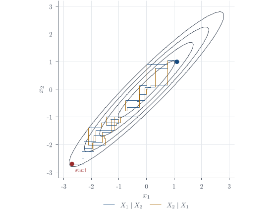
Discarding early draws is called warm-up or burn-in. It limits dependence on the chosen initial state, but it is not a proof of convergence. Strong posterior correlation produces staircase-like Gibbs paths and high autocorrelation. Separated modes are harder still because a coordinate-wise move may have to cross a low-density barrier.
Thinning by retaining every kth draw reduces storage and visible serial dependence, but usually throws away usable information. Unless storage or an expensive downstream calculation is the constraint, retain all post-warm-up draws and quantify their effective sample size. Posterior means, probabilities, and equal-tailed intervals are computed from those draws; a continuous MAP is found by optimisation, not by asking which simulated value occurred most often.
Examples
Bivariate exponential target
Worked example from Markov chains, Gibbs sampling, and Metropolis–Hastings
The target is
\pi(x_1,x_2)\propto e^{-x_1x_2-x_1-x_2}, \qquad x_1,x_2\geq0.
Question. Derive both full conditional distributions and use them to specify a systematic-scan Gibbs sampler.
Solution. To obtain X_1\mid X_2=x_2, hold x_2 fixed: \begin{align*} \pi(x_1\mid x_2) &\propto\pi(x_1,x_2)\\ &\propto e^{-x_1x_2-x_1-x_2}\\ &\propto e^{-x_1(x_2+1)}, \qquad x_1\geq0. \end{align*} The omitted factor e^{-x_2} is constant in x_1. Normalising gives
\pi(x_1\mid x_2)=(x_2+1)e^{-(x_2+1)x_1},
so
X_1\mid X_2=x_2\sim\operatorname{Exp}(x_2+1).
By symmetry,
X_2\mid X_1=x_1\sim\operatorname{Exp}(x_1+1).
Starting from any nonnegative pair (x_1^{(0)},x_2^{(0)}), the sampler is \begin{align*} x_1^{(t+1)}&\sim\operatorname{Exp}(x_2^{(t)}+1),\\ x_2^{(t+1)}&\sim\operatorname{Exp}(x_1^{(t+1)}+1). \end{align*}
Normal mean and variance
Worked example from Markov chains, Gibbs sampling, and Metropolis–Hastings
Question. For the joint normal-model posterior in Equation (4) in Conjugate analysis for normal models, describe a systematic Gibbs sampler and state how retained draws estimate the posterior mean of \mu.
Solution. For the joint posterior in Equation (4) in Conjugate analysis for normal models, alternate \begin{align*} \mu^{(t+1)}&\sim p(\mu\mid\sigma^{2(t)},{\boldsymbol{x}}) \quad\text{using (5)},\\ \sigma^{2(t+1)}&\sim p(\sigma^2\mid\mu^{(t+1)},{\boldsymbol{x}}) \quad\text{using (6)}. \end{align*} After discarding a warm-up segment, Monte Carlo estimates use the retained draws. For example,
\widehat{\mathbb{E}}(\mu\mid{\boldsymbol{x}}) =\frac1L\sum_{t=B+1}^{B+L}\mu^{(t)},
where B is the number of discarded iterations. Because the draws are dependent, L correlated draws contain less information than L independent draws. Autocorrelation, trace plots, multiple chains, and effective sample size are therefore part of a serious analysis.
Q4. Gibbs sampling from full conditionals
Question page: Q4. Gibbs sampling from full conditionals
Let X\in\{0,1,\ldots,10\} and 0<\theta<1 have joint density/mass function \pi(x,\theta) \propto \binom{10}{x}\theta^{x+1}(1-\theta)^{12-x}.
(a) [2 marks] Find and identify the conditional distribution of X\mid\theta.
(b) [2 marks] Find and identify the conditional distribution of \theta\mid X=x.
(c) [3 marks] Hence write pseudocode for a Gibbs sampler that generates a Markov chain with equilibrium distribution \pi(x,\theta). Begin from an arbitrary valid starting value (x^{(0)},\theta^{(0)}).
(d) [2 marks] Explain why there is no accept-reject step in this Gibbs sampler.
(e) [1 mark] Are the resulting pairs \bigl(X^{(1)},\theta^{(1)}\bigr), \bigl(X^{(2)},\theta^{(2)}\bigr),\ldots independent? Briefly explain.
Definitions. A full conditional is obtained by normalising the joint in the variable being updated; the other variable is fixed. The relevant kernels are \operatorname{Bin}(n,p):\ \binom nx p^x(1-p)^{n-x},\quad x=0,\ldots,n, \operatorname{Beta}(a,b):\ u^{a-1}(1-u)^{b-1},\quad 0<u<1,\quad a,b>0. Here n=10; superscript (t) denotes a completed Gibbs iteration.
(a) Conditional distribution of X\mid\theta
Holding \theta fixed and retaining the terms that depend on x, \begin{aligned} \pi(x\mid\theta) &\propto \binom{10}{x}\theta^{x+1}(1-\theta)^{12-x}\\ &=\theta(1-\theta)^2 \binom{10}{x}\theta^x(1-\theta)^{10-x}\\ &\propto \binom{10}{x}\theta^x(1-\theta)^{10-x}. \end{aligned} The discarded factor \theta(1-\theta)^2 is constant with respect to x. Therefore, \boxed{X\mid\theta\sim\operatorname{Bin}(10,\theta)}.
(b) Conditional distribution of \theta\mid X=x
Holding x fixed, \pi(\theta\mid x) \propto \theta^{x+1}(1-\theta)^{12-x}, \qquad 0<\theta<1. The kernel of a \operatorname{Beta}(\alpha,\beta) distribution is \theta^{\alpha-1}(1-\theta)^{\beta-1}. Matching powers gives \alpha=x+2, \qquad \beta=13-x. Hence, \boxed{ \theta\mid X=x \sim\operatorname{Beta}(x+2,13-x) }.
(c) Gibbs-sampler pseudocode
Choose any valid starting values x^{(0)}\in\{0,1,\ldots,10\}, \qquad \theta^{(0)}\in(0,1). For t=1,2,\ldots,T:
1. Generate X^{(t)} \sim\operatorname{Bin}\bigl(10,\theta^{(t-1)}\bigr).
2. Using the newly generated X^{(t)}, generate \theta^{(t)} \sim\operatorname{Beta}\bigl(X^{(t)}+2,13-X^{(t)}\bigr).
3. Store \bigl(X^{(t)},\theta^{(t)}\bigr).
After a suitable burn-in, the stored states have approximately the target equilibrium distribution \pi(x,\theta).
(d) Why there is no accept-reject step
Each update is sampled directly from its exact full conditional distribution. The generated value therefore already has the required conditional distribution and is always accepted. Equivalently, Gibbs sampling is a special case of Metropolis-Hastings whose acceptance probability is 1.
(e) Independence of the sampled pairs
No. The update X^{(t)} depends on \theta^{(t-1)}, and \theta^{(t)} then depends on X^{(t)}. Successive states therefore form a Markov chain and are generally serially dependent. Once the chain is in equilibrium, each individual state has marginal distribution \pi(x,\theta), but this does not make the states independent.
Key result. The two full conditionals are \boxed{ X\mid\theta\sim\operatorname{Bin}(10,\theta), \qquad \theta\mid X=x\sim\operatorname{Beta}(x+2,13-x) }. At each iteration, sample from these in order using the newest available value. Exact full-conditional draws require no rejection, but successive Gibbs states are not independent.
Q9. Gibbs sampling for a correlated normal target
Question page: Q9. Gibbs sampling for a correlated normal target
Consider the joint posterior density p(\theta_1,\theta_2\mid{\boldsymbol{x}}) \propto \exp\left[ -\frac{\theta_1^2-2\rho\theta_1\theta_2+\theta_2^2} {2(1-\rho^2)} \right], where \theta_1,\theta_2\in\mathbb{R} and -1<\rho<1 is known.
(a) Derive the two full conditional distributions, identifying their means and variances. [4 marks]
(b) Give pseudocode for a Gibbs sampler with this equilibrium density. Make clear which current or updated value is used at each step. [3 marks]
(c) Suppose the initial pair is drawn exactly from the equilibrium distribution. Are the subsequent sampled pairs necessarily independent? Explain. [2 marks]
(d) When \rho is close to 1, explain why this sampler may move slowly through the joint posterior, even though every Gibbs update is accepted. [3 marks]
Definitions. The target coordinates \theta_1,\theta_2 have zero means, unit marginal variances, and correlation \rho, with -1<\rho<1. A full conditional holds the other coordinate and the data x fixed. The Normal kernel \exp\{-(u-m)^2/(2v)\} identifies mean m and variance v>0. Superscript (t) labels the Gibbs sweep.
The joint density has kernel \pi(\theta_1,\theta_2\mid x) \propto \exp\left\{ -\frac{1}{2(1-\rho^2)} \left(\theta_1^2-2\rho\theta_1\theta_2+\theta_2^2\right) \right\}.
(a) Full conditional distributions
For the first full conditional, p(\theta_1\mid\theta_2,x) = \frac{p(\theta_1,\theta_2\mid x)}{p(\theta_2\mid x)} \propto p(\theta_1,\theta_2\mid x) \quad\text{as a function of }\theta_1. The denominator is constant when \theta_2 and x are held fixed. Thus the joint kernel is sufficient: terms involving \theta_1 must be kept, while terms free of \theta_1 may be absorbed into the proportionality constant.
We aim to match the Normal kernel \exp\left\{-\frac{(\theta_1-m)^2}{2v}\right\}, where m is the mean and v is the variance. Treat the quadratic form in the joint exponent as a quadratic in \theta_1. Completing the square gives \begin{aligned} \theta_1^2-2\rho\theta_1\theta_2+\theta_2^2 &=(\theta_1-\rho\theta_2)^2 -\rho^2\theta_2^2+\theta_2^2\\ &=(\theta_1-\rho\theta_2)^2 +(1-\rho^2)\theta_2^2. \end{aligned} Substitution into the joint kernel gives \begin{aligned} p(\theta_1\mid\theta_2,x) &\propto \exp\left\{ -\frac{(\theta_1-\rho\theta_2)^2+(1-\rho^2)\theta_2^2} {2(1-\rho^2)} \right\}\\ &= \exp\left\{-\frac{(\theta_1-\rho\theta_2)^2} {2(1-\rho^2)}\right\} \exp\left\{-\frac{\theta_2^2}{2}\right\}\\ &\propto \exp\left\{-\frac{(\theta_1-\rho\theta_2)^2} {2(1-\rho^2)}\right\}. \end{aligned} The factor \exp(-\theta_2^2/2) is dropped because it is constant with respect to \theta_1. Matching the remaining expression to the Normal kernel yields \boxed{ \theta_1\mid\theta_2,x \sim N\left(\rho\theta_2,\,1-\rho^2\right). } The condition -1<\rho<1 ensures that the conditional variance 1-\rho^2 is positive.
For the other coordinate, the same calculation gives \theta_2^2-2\rho\theta_1\theta_2+\theta_1^2 = (\theta_2-\rho\theta_1)^2+(1-\rho^2)\theta_1^2. Hence, by symmetry, \boxed{ \theta_2\mid\theta_1,x \sim N\left(\rho\theta_1,\,1-\rho^2\right). }
(b) Gibbs sampler
Starting from any valid pair (\theta_1^{(0)},\theta_2^{(0)})\in\mathbb{R}^2, repeat for t=1,\ldots,T:
1. Draw \theta_1^{(t)} \sim N\left(\rho\theta_2^{(t-1)},\,1-\rho^2\right).
2. Draw \theta_2^{(t)} \sim N\left(\rho\theta_1^{(t)},\,1-\rho^2\right).
3. Store (\theta_1^{(t)},\theta_2^{(t)}).
Each update is sampled directly from a full conditional distribution, so no accept–reject step is required.
(c) Equilibrium and independence
If the chain is started in equilibrium, every stored pair has the required joint distribution. The pairs are nevertheless generally not independent, because the distribution of the next pair depends on the current pair through the Gibbs updates.
When \rho=0, the coordinates are independent and fresh conditional draws produce independent pairs across full sweeps. This exception does not apply to a correlated target.
(d) Effect of strong correlation
When \rho is close to 1, the joint density is concentrated around the diagonal \theta_1=\theta_2, while the conditional variance 1-\rho^2 is close to zero. Each Gibbs update therefore makes only a small move along the narrow high-density region. This produces strong autocorrelation and slow mixing. Thus, although every Gibbs proposal is accepted, an acceptance rate of one does not imply efficient exploration of the target distribution.
Question 6. Geometric–beta Gibbs sampler
Question page: Question 6. Geometric–beta Gibbs sampler
Consider X and Y with joint density
f(x,y)\propto y^{\alpha}(1-y)^{x+\beta-1},
for x=1,2,3,\ldots and 0<y<1, where \alpha>0 and \beta>0. Describe a Gibbs sampler for this joint density.
Definitions. This target has one discrete coordinate X\in\{1,2,\ldots\} and one continuous coordinate Y\in(0,1). Here \operatorname{Geom}(p) counts trials up to and including the first success, with mass p(1-p)^{x-1}. A \operatorname{Beta}(a,b) density is proportional to y^{a-1}(1-y)^{b-1}. When finding a full conditional, keep all factors involving the coordinate being updated and normalise over that coordinate’s support.
For 0<y<1, the factors in x are (1-y)^{x-1}. For r=1-y\in(0,1),
\sum_{x=1}^{\infty}r^{x-1}=\frac{1}{1-r}=\frac{1}{y},
so
X\mid y\sim\operatorname{Geom}(y), \qquad \mathbb{P}(X=x\mid y)=y(1-y)^{x-1},\quad x=1,2,\ldots.
The factors in y are y^{(\alpha+1)-1}(1-y)^{(x+\beta)-1}, so
Y\mid x\sim\operatorname{Beta}(\alpha+1,\,x+\beta).
Record the completed pair. Each draw is from an exact full conditional, so there is no acceptance step. To see why an update preserves the joint target, suppose a pair already has density f: leaving Y unchanged and redrawing X from f(x\mid Y) gives f_Y(y)f(x\mid y)=f(x,y) again. The same reasoning applies to the other coordinate and hence to their composition. Convergence from the chosen start still needs assessment, and successive sweeps are generally dependent.
The target is proper: summing its kernel over x leaves y^{\alpha-1}(1-y)^\beta, which has a finite beta integral for the stated positive parameters. In fact, this also identifies Y\sim\operatorname{Beta}(\alpha,\beta+1) marginally. It provides a useful check on a Gibbs simulation; it is different from the full conditional Y\mid X.
Support and mixing checks. Correct full conditionals alone do not guarantee useful exploration. For example, take a target uniform on the two disjoint squares (0,1)^2 and (2,3)^2. Updating one coordinate while holding the other fixed cannot leave the current square, so a single-coordinate Gibbs chain cannot explore the whole target. The present geometric–beta target is positive over its product support and has no such hard separation. Strong dependence can nevertheless make exploration slow; a longer discarded prefix does not fix poor mixing. If implementing the first draw with R’s rgeom, add one because R counts failures before success.
Used in
- Taught in Markov chains, Gibbs sampling, and Metropolis–Hastings, where the derivation and examples are.
- Also used in Markov chains · Conjugate analysis for normal models · Exponential families and conjugacy · Hierarchical Bayes · Bayesian linear regression · Reference formulas and problem-solving workflow
- Questions that use it (24) — A bivariate-normal Gibbs sampler · Direct sampling or Gibbs? · Independent and scaled priors · Q4 · Q9 · Q14 · Q18 · Q23 · Q25 · Q26 · Q43 · Q49 · Q51 · Q58 · Q59 · Question 3 · Question 5 · Question 6 · Question 9 · Question 12 (answer) · Question 13 · Question 16 · Question 17 · C13
- All 31 questions on Markov chains, Gibbs sampling, and Metropolis–Hastings
See also
Joint probability density · Three easy confusions · Markov chain · Stationarity and detailed balance · Detailed balance implies stationarity · Warm-up is not a convergence proof · Metropolis–Hastings update · Metropolis–Hastings invariance