Question 16. Mixed binomial–beta Gibbs sampler
Topic: Markov chains, Gibbs sampling, and Metropolis–Hastings · more questions on this topic
‹ Question 13 C11 ›
Consider the mixed probability function
f(x,y,z)\propto \binom{n}{x}\binom{m}{y} z^{x+y+\alpha-1}(1-z)^{n+m-x-y+\beta-1} \gamma^{m-y}(1-\gamma)^{n-x}\delta^{x}(1-\delta)^{y},
for x=0,1,\ldots,n, y=0,1,\ldots,m, and 0<z<1, where \alpha,\beta>0 and 0<\gamma,\delta<1. Identify the full conditionals and give a Gibbs sampler; implement and run it for 100{,}000 iterations, reporting marginal plots and summaries; and, for \alpha=2, \beta=4, \gamma=0.3, \delta=0.6, n=10, and m=20, apply conditional-mode updates until they no longer change.
Definitions. X and Y are bounded counts, while Z is a probability in (0,1). The positive values \alpha,\beta and probabilities \gamma,\delta are fixed hyperparameters. A full conditional holds the other two coordinates fixed. A conditional mode maximises that conditional distribution; replacing random draws by modes produces a deterministic optimisation procedure rather than a sampler.
The question gives numerical values only for the mode updates, and it gives no initial state. The run and the mode iteration below use those values and the initial state (x,y,z)=(5,10,1/2).
Full conditionals. Write q for the displayed kernel, so f=q/C on x\in\{0,\ldots,n\}, y\in\{0,\ldots,m\} and z\in(0,1). A full conditional is q renormalised in the target coordinate. Factors free of that coordinate cancel.
For x, split (1-z)^{n+m-x-y+\beta-1}=(1-z)^{n-x}(1-z)^{m-y+\beta-1}. The factors containing x are
\binom{n}{x}(z\delta)^{x}\bigl[(1-z)(1-\gamma)\bigr]^{n-x}.
For z\in(0,1) and \gamma,\delta\in(0,1), both A_x=z\delta and B_x=(1-z)(1-\gamma) are positive. Then
\binom{n}{x}A_x^{x}B_x^{n-x} = (A_x+B_x)^{n} \binom{n}{x}p_x^{x}(1-p_x)^{n-x}, \quad p_x=\frac{A_x}{A_x+B_x},
and (A_x+B_x)^{n} does not depend on x. Therefore
\boxed{X\mid y,z \sim \operatorname{Bin}\!\left(n,\ \frac{z\delta}{z\delta+(1-z)(1-\gamma)}\right).}
This conditional does not depend on y.
For y, split (1-z)^{n+m-x-y+\beta-1}=(1-z)^{m-y}(1-z)^{n-x+\beta-1}. The factors containing y are
\binom{m}{y}\bigl[z(1-\delta)\bigr]^{y}\bigl[(1-z)\gamma\bigr]^{m-y}.
The same binomial argument, with both bases positive, gives
\boxed{Y\mid x,z \sim \operatorname{Bin}\!\left(m,\ \frac{z(1-\delta)}{z(1-\delta)+(1-z)\gamma}\right).}
This conditional does not depend on x.
For z, the factors containing z are z^{x+y+\alpha-1}(1-z)^{n+m-x-y+\beta-1} on (0,1). Since \alpha,\beta>0 and 0\le x\le n, 0\le y\le m,
a_z:=x+y+\alpha>0, \qquad b_z:=n+m-x-y+\beta>0.
This is the \operatorname{Beta}(a_z,b_z) kernel, whose integral is the beta function \mathrm{B}(a_z,b_z). Hence
\boxed{Z\mid x,y \sim \operatorname{Beta}(x+y+\alpha,\ n+m-x-y+\beta).}
Gibbs sampler. Let p_X(z) and p_Y(z) be the success probabilities derived above.
The two binomial draws both use the previous sweep’s z, and neither uses the other count. The beta draw uses both new counts. This is consistent with sequential Gibbs updating because the count conditionals do not depend on each other. Each draw stays within its stated support. Check mixing before summarising the retained triples; the deterministic mode updates below do not replace this sampling step.
In fact, X and Y are conditionally independent given Z: at a fixed z, the joint kernel factors into a function of x and a function of y. They need not be independent marginally, since both success probabilities vary with the shared Z. Recording only one coordinate from the joint chain approximates its marginal distribution, automatically averaging over the other coordinates.
Run. Use \alpha=2, \beta=4, \gamma=0.3, \delta=0.6, n=10, m=20, and the sweeps above, for 100{,}000 iterations from (5,10,1/2), with generator seed 3500. Discard the first 1{,}000 iterations. The marginal summaries of the remaining 99{,}000 draws are
| mean | sd | 2.5\% | 50\% | 97.5\% | |
|---|---|---|---|---|---|
| x | 4.498 | 2.349 | 0 | 4 | 9 |
| y | 10.880 | 4.264 | 2 | 11 | 18 |
| z | 0.483 | 0.186 | 0.119 | 0.487 | 0.822 |
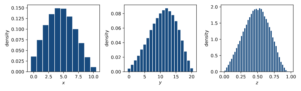
Conditional modes. For 0<p<1 and k=1,\ldots,n,
\frac{\mathbb{P}(W=k)}{\mathbb{P}(W=k-1)} = \frac{n-k+1}{k}\cdot\frac{p}{1-p} \ge 1 \iff k\le (n+1)p,
when W\sim\operatorname{Bin}(n,p). Thus the pmf is maximised at \lfloor(n+1)p\rfloor. If (n+1)p is an integer, that value and the integer one smaller are both modes.
For the beta coordinate, a=x+y+\alpha\ge 2>1 and b=n+m-x-y+\beta\ge 4>1 at these parameter values, for every feasible (x,y). The log conditional density has derivative (a-1)/z-(b-1)/(1-z) and second derivative -(a-1)/z^{2}-(b-1)/(1-z)^{2}<0, so the conditional mode is
z=\frac{a-1}{a+b-2} = \frac{x+y+\alpha-1}{n+m+\alpha+\beta-2} = \frac{x+y+1}{34}.
Update in the Gibbs order, using the latest value of each conditioning variable. At a binomial tie, take the larger mode \lfloor(n+1)p\rfloor. Starting at (5,10,1/2), with \delta=3/5 and \gamma=3/10,
p_X(1/2)=\frac{6}{13}, \qquad 11\cdot\frac{6}{13}=\frac{66}{13}\notin\mathbb{Z},
so the x-mode is 5. Also
p_Y(1/2)=\frac{4}{7}, \qquad 21\cdot\frac{4}{7}=12\in\mathbb{Z},
so y has modes 11 and 12. The larger mode is 12, and then
z=\frac{5+12+1}{34}=\frac{9}{17}.
At this state,
p_X(9/17)=\frac{27}{55}, \quad 11\cdot\frac{27}{55}=\frac{27}{5}, \quad \lfloor 27/5\rfloor=5,
and
p_Y(9/17)=\frac{3}{5}, \quad 21\cdot\frac{3}{5}=\frac{63}{5}, \quad \lfloor 63/5\rfloor=12,
neither success probability giving an integer (n+1)p. The beta mode is again 9/17.
\therefore \text{the iteration stops at } \Bigl(5,\ 12,\ \tfrac{9}{17}\Bigr).
Note: selecting the smaller y-mode at the tie stops at (5,11,1/2) instead. Other initial states can stop at other conditional-mode fixed points.
Each mode update can only increase or preserve the joint density with the other coordinates fixed. That explains the coordinate-ascent interpretation, but it does not prove that the terminal point is a global joint mode. More importantly, these terminal values do not quantify marginal uncertainty: the simulated spread and quantiles above come from random full-conditional draws, not from the mode iteration. Warm-up removal is a starting-point precaution; trace plots and autocorrelation checks are still needed to assess the simulation.