Credible-region constructions
Definition taught in Bayesian foundations, part of Bayesian statistics
Credible-region constructions
| Type | Definition |
| Taught in | Bayesian foundations |
| Part | Bayesian statistics |
| Properties | 1 |
| Worked examples | 2 |
| Questions using it | 4 |
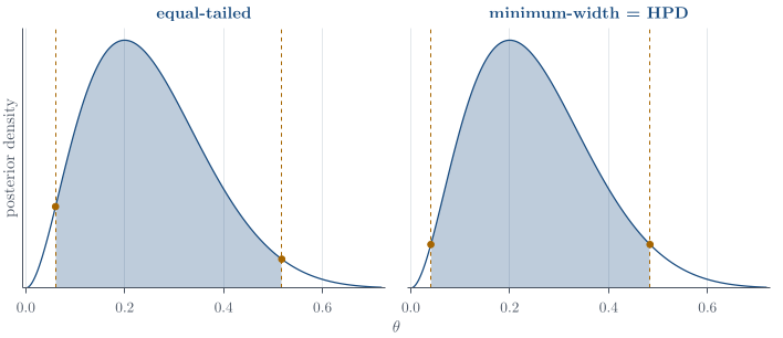
Three interval constructions are worth distinguishing. An equal-tailed 95\% credible interval (l,u) satisfies
\mathbb{P}(\theta<l\mid x)=0.025, \qquad \mathbb{P}(\theta>u\mid x)=0.025.
The minimum-width interval solves
\min_{l<u}(u-l) \quad\text{subject to}\quad \int_l^u p(\theta\mid x)\,\mathrm{d}\theta=0.95.
A highest-posterior-density set chooses a level c so that
\mathcal H_c=\{\theta:p(\theta\mid x)\geq c\}, \qquad \int_{\mathcal H_c}p(\theta\mid x)\,\mathrm{d}\theta=0.95.
Every included point then has density at least as large as every excluded point. For a continuous unimodal posterior this gives the minimum-width interval; for a multimodal posterior the highest-density set can be disjoint. For a symmetric unimodal density, the mean, median, and mode coincide and the common interval constructions often agree.
Properties
Posterior summaries from draws
Main article: Posterior summaries from draws
Let \theta^{(1)},\ldots,\theta^{(L)} be posterior draws and let \theta_{(1)}\leq\cdots\leq\theta_{(L)} be their order statistics. Then \begin{align*} \widehat{\mathbb{E}}(\theta\mid x) &=\frac1L\sum_{l=1}^L\theta^{(l)},\\ \widehat{\operatorname{Var}}(\theta\mid x) &=\frac1{L-1}\sum_{l=1}^L \left(\theta^{(l)}-\overline\theta\right)^2,\\ \widehat{\mathbb{P}}(\theta<c\mid x) &=\frac1L\sum_{l=1}^L\mathbf{1}\{\theta^{(l)}<c\}. \end{align*} The posterior median and equal-tailed interval are estimated by the corresponding empirical quantiles. With L=1000, the median can be estimated by the average of \theta_{(500)} and \theta_{(501)}, and a direct 95\% interval approximation by [\theta_{(25)},\theta_{(975)}]. The precise indices vary slightly with a software package’s quantile convention.
Examples
Q8. Equal-tailed and highest-density intervals
Question page: Q8. Equal-tailed and highest-density intervals
Suppose a continuous parameter \theta has posterior density p(\theta\mid{\boldsymbol{x}})=2\theta, \qquad 0<\theta<1, and zero elsewhere.
(a) Find a 75% equal-tailed posterior credible interval. [3 marks]
(b) Find a minimum-width 75% posterior credible interval. Sketch the posterior density and explain why your interval is a highest-density interval. Exact expressions are sufficient. [3 marks]
(c) A frequentist confidence-interval procedure happens to return the same endpoints as one of your intervals. Explain the difference between a 75% confidence statement and a 75% posterior credible statement. [2 marks]
Definitions. For a continuous posterior, F(u)=\mathbb P(\theta\le u\mid{\boldsymbol{x}}) and F^{-1} is its quantile function. An equal-tailed interval puts half the omitted probability in each tail. A highest-density interval (HDI, also called HPD) includes points of at least as high density as those excluded. Here the posterior density is 2\theta on (0,1) and the required probability is 0.75.
For 0<\theta<1, the posterior distribution function is F(\theta)=\int_0^\theta 2u\,du=\theta^2, \qquad F^{-1}(p)=\sqrt{p}.
(a) Equal-tailed 75% credible interval
An equal-tailed 75% interval leaves probability 0.125 in each tail. Therefore its endpoints are F^{-1}(0.125)=\sqrt{\frac18}, \qquad F^{-1}(0.875)=\sqrt{\frac78}. Thus \boxed{ \left[\sqrt{\frac18},\sqrt{\frac78}\right] } is the 75% equal-tailed posterior credible interval.
(b) Minimum-width 75% credible interval
The posterior density 2\theta increases throughout (0,1), so the highest-density interval must contain the largest values of \theta and end at 1. Let it be [c,1]. Then \mathbb{P}(c\leq\theta\leq1\mid{\boldsymbol{x}}) =1-F(c)=1-c^2=0.75, which gives c=1/2. Hence the minimum-width interval is \boxed{\left[\frac12,1\right]}.
Every included point has density at least as large as every excluded point, so [1/2,1] is a highest-density interval. Equivalently, among intervals [a,b] satisfying b^2-a^2=0.75, its width (b-a)=0.75/(a+b) is minimised by taking the largest possible a+b, namely b=1 and a=1/2.
(c) Confidence versus credibility
A 75% confidence procedure has repeated-sampling coverage \mathbb{P}_{\theta}\{L(X)\leq\theta\leq U(X)\}=0.75. The probability refers to the random interval procedure; after observing the data, the realised frequentist interval is fixed.
A 75% credible interval [a,b] satisfies \mathbb{P}(a\leq\theta\leq b\mid{\boldsymbol{x}})=0.75. This probability refers directly to the posterior distribution of \theta given the observed data, prior, and model. Identical numerical endpoints do not change these different interpretations.
Q13. Bayesian German tank problem
Question page: Q13. Bayesian German tank problem
In the Second World War, Allied statisticians estimated German tank production from the serial numbers on captured tanks. Treat the serial numbers as continuous. Suppose X_1,\ldots,X_n\mid\theta \overset{\mathrm{iid}}{\sim}\operatorname{Uniform}(0,\theta), \qquad \theta>0, and write x_{(n)}=\max_i x_i. Place the Pareto prior p(\theta\mid\alpha,\beta) =\frac{\alpha\beta^\alpha}{\theta^{\alpha+1}}, \qquad \theta\geq\beta, where \alpha,\beta>0. Here \beta is a known lower bound on production.
[13 marks]
(a) Write the likelihood with every indicator function shown explicitly. Derive the posterior distribution of \theta and show that it is Pareto. State its parameters, and state exactly when the data change the prior lower bound. [4 marks]
(b) Find the posterior mean. The MLE is \widehat{\theta}_{\mathrm{MLE}}=x_{(n)}. Explain why the posterior mean always exceeds it, and why this is sensible rather than a sign of bias in the Bayesian estimate. [2 marks]
(c) Derive the posterior predictive density of one new captured serial number \widetilde X. Show that it is a two-component mixture, and identify both components and their weights. Find \mathbb{P}\!\left( \widetilde X>\max\{\beta,x_{(n)}\}\mid{\boldsymbol{x}} \right) and interpret it. [4 marks]
(d) The Pitman–Koopman–Darmois theorem links sufficient statistics of fixed dimension to exponential families. Here x_{(n)} is a one-dimensional sufficient statistic for every n, and a conjugate prior exists. Explain why this does not make \operatorname{Uniform}(0,\theta) an exponential family, and why it does not contradict the theorem. [2 marks]
(e) The captured serials are 19,40,42,60, and the prior has \alpha=1 and \beta=50. Give the posterior mean and a 95% highest-posterior-density interval for \theta. Justify the lower endpoint of the interval. [1 mark]
Definitions. Write x_{(1)}=\min_i x_i and x_{(n)}=\max_i x_i; \mathbf1\{A\} is one when A holds and zero otherwise. Our Pareto convention is p(\theta)=ab^a\theta^{-a-1}\mathbf1\{\theta\ge b\}, with shape a>0 and lower bound b>0. \widetilde X denotes a new serial number, conditionally independent of the sample given \theta. We use the stated continuous, conditionally iid model with n\ge1 and positive observations.
Write a_n=\alpha+n, \qquad b_n=\max\{\beta,x_{(n)}\}.
(a) Likelihood and posterior
For observations from \operatorname{Uniform}(0,\theta), \begin{aligned} L(\theta;{\boldsymbol{x}}) &=\prod_{i=1}^n \left[\frac{1}{\theta}\, \mathbf{1}\{0<x_i<\theta\}\right]\\ &=\theta^{-n}\, \mathbf{1}\{x_{(1)}>0\} \prod_{i=1}^n\mathbf{1}\{x_i<\theta\}\\ &=\theta^{-n}\, \mathbf{1}\{x_{(1)}>0\} \mathbf{1}\{x_{(n)}<\theta\}. \end{aligned} For a valid observed sample, \mathbf{1}\{x_{(1)}>0\} does not depend on \theta. Hence L(\theta;{\boldsymbol{x}}) \propto\theta^{-n}\mathbf{1}\{\theta>x_{(n)}\}. Multiplying by the prior gives \begin{aligned} p(\theta\mid{\boldsymbol{x}}) &\propto \theta^{-n}\mathbf{1}\{\theta>x_{(n)}\} \theta^{-(\alpha+1)}\mathbf{1}\{\theta\geq\beta\}\\ &=\theta^{-(\alpha+n+1)} \mathbf{1}\{\theta\geq b_n\}\\ &=\theta^{-(a_n+1)}\mathbf{1}\{\theta\geq b_n\}. \end{aligned} The distinction between strict and non-strict inequalities at one endpoint is irrelevant for a continuous density. Since \int_{b_n}^{\infty}\theta^{-(a_n+1)}\,d\theta =\frac{b_n^{-a_n}}{a_n}, the normalised posterior density is p(\theta\mid{\boldsymbol{x}}) =\frac{a_n b_n^{a_n}}{\theta^{a_n+1}}, \qquad \theta\geq b_n. Therefore, \boxed{ \theta\mid{\boldsymbol{x}} \sim\operatorname{Pareto}\!\left( \alpha+n,\max\{\beta,x_{(n)}\} \right). } The data change the lower bound exactly when x_{(n)}>\beta. Otherwise the lower bound remains \beta, although the shape still changes from \alpha to \alpha+n.
(b) Posterior mean
Because a_n=\alpha+n>1, the posterior mean exists and is \boxed{ \mathbb{E}(\theta\mid{\boldsymbol{x}}) =\frac{a_n b_n}{a_n-1} =\frac{(\alpha+n)\max\{\beta,x_{(n)}\}} {\alpha+n-1}. } Since a_n/(a_n-1)>1 and b_n\geq x_{(n)}, \mathbb{E}(\theta\mid{\boldsymbol{x}})>b_n\geq x_{(n)} =\widehat{\theta}_{\mathrm{MLE}}. This is sensible. The MLE is the smallest value of \theta compatible with the data because the likelihood decreases for \theta>x_{(n)}. Moreover, X_{(n)}<\theta almost surely and \mathbb{E}(X_{(n)}\mid\theta)=\frac{n}{n+1}\theta, so the sample maximum systematically falls below the true upper endpoint. The posterior mean allows for the unobserved region above the largest captured serial. Frequentist bias is a repeated-sampling property; the posterior mean is instead the Bayes estimate under squared-error loss.
(c) Posterior predictive distribution
For a new serial number \widetilde X, \begin{aligned} p(\widetilde x\mid{\boldsymbol{x}}) &=\int_{b_n}^{\infty} \frac{1}{\theta}\mathbf{1}\{0<\widetilde x<\theta\} \frac{a_n b_n^{a_n}}{\theta^{a_n+1}}\,d\theta\\ &=a_n b_n^{a_n} \int_{\max\{b_n,\widetilde x\}}^{\infty} \theta^{-(a_n+2)}\,d\theta, \qquad \widetilde x>0. \end{aligned} Thus p(\widetilde x\mid{\boldsymbol{x}}) = \begin{cases} \displaystyle \frac{a_n}{a_n+1}\frac{1}{b_n}, &0<\widetilde x\leq b_n,\\[1.1em] \displaystyle \frac{a_n b_n^{a_n}}{(a_n+1)\widetilde x^{a_n+1}}, &\widetilde x>b_n,\\[0.8em] 0,&\widetilde x\leq0. \end{cases} Equivalently, this is the mixture \boxed{ \frac{a_n}{a_n+1}\operatorname{Uniform}(0,b_n) +\frac{1}{a_n+1}\operatorname{Pareto}(a_n,b_n). } The component weights sum to one. The Uniform component has no probability above b_n, whereas the Pareto component lies above b_n almost surely. Therefore, \boxed{ \mathbb{P}(\widetilde X>b_n\mid{\boldsymbol{x}}) =\frac{1}{a_n+1} =\frac{1}{\alpha+n+1}. } This is the posterior predictive probability that the next captured serial exceeds whichever is larger: the confirmed lower bound \beta or the current sample maximum.
(d) Why there is no contradiction with the Pitman–Koopman–Darmois theorem
In a regular exponential-family model, the support cannot change with the parameter: a representation of the form p(x\mid\theta) =b(x)\frac{\exp\{c(\theta)T(x)\}}{a(\theta)} has support determined by b(x), since the exponential term is positive. For the Uniform model, p(x\mid\theta)=\frac{1}{\theta} \mathbf{1}\{0<x<\theta\}, and the indicator switches on or off as \theta changes. Its support depends on \theta, so this is an irregular model rather than a regular exponential family.
The Pitman–Koopman–Darmois theorem assumes, among other regularity conditions, parameter-independent support. This model violates that assumption and lies outside the theorem’s scope. It may therefore have the fixed-dimensional sufficient statistic x_{(n)} and a conjugate prior without being an exponential family. The existence of a conjugate prior does not by itself imply exponential-family structure.
(e) Numerical posterior and 95% HPD interval
Here n=4, x_{(n)}=60, \alpha=1, and \beta=50, so a_n=5, \qquad b_n=60, \qquad \theta\mid{\boldsymbol{x}}\sim\operatorname{Pareto}(5,60). The posterior mean is \boxed{ \mathbb{E}(\theta\mid{\boldsymbol{x}})=\frac{5(60)}{4}=75. } The posterior density is strictly decreasing on [60,\infty), so its highest-density interval must begin at the posterior mode and lower support boundary, 60. If the upper endpoint is u, then 0.05 =\mathbb{P}(\theta>u\mid{\boldsymbol{x}}) =\left(\frac{60}{u}\right)^5. Hence u=60(20)^{1/5}\approx109.2, and \boxed{ \text{95\% HPD interval} =\left[60,\,60(20)^{1/5}\right] \approx[60,109.2]. } The lower endpoint is 60 because values below the largest observed serial are impossible, and the decreasing posterior density is maximised at that boundary.
Used in
- Taught in Bayesian foundations, where the derivation and examples are.
- Also used in Markov chains, Gibbs sampling, and Metropolis–Hastings · Reference formulas and problem-solving workflow
- Questions that use it (4) — An IQ threshold (answer) · Q8 · Q13 · Q28 (answer)
- All 15 questions on Bayesian foundations
See also
Bayesian credible interval · Posterior summaries from draws · R’s distribution interface · Warm-up is not a convergence proof · Bayes’ rule · Proper prior and proper posterior · Posterior point summaries · Prior and posterior predictive distributions