Exponential distribution
Definition taught in Random variables and distributions, part of Probability · Also on the distribution sheet
Exponential distribution
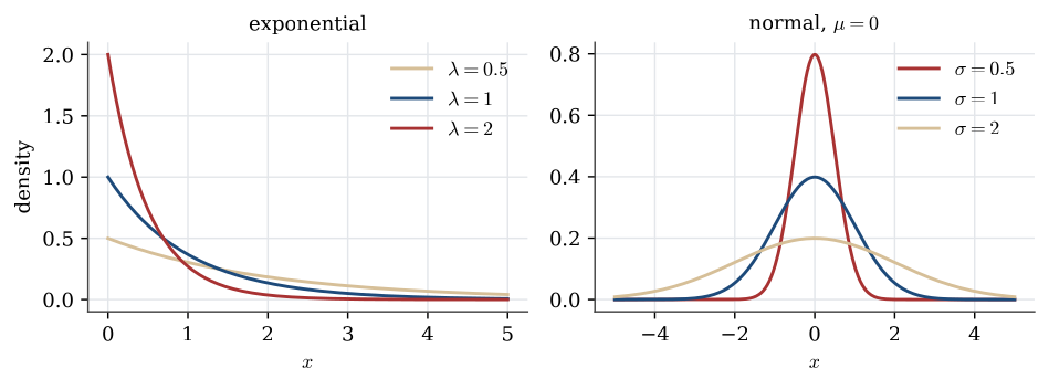
| Notation | x\sim\operatorname{Exp}(\lambda) |
| Parameters | \lambda>0 |
| Support | x>0 |
| Density | p(x)=\lambda e^{-\lambda x} |
| Mean | \mathbb{E}(x)=1/\lambda |
| Variance | \operatorname{Var}(x)=1/\lambda^{2} |
| Taught in | Random variables and distributions |
| Part | Probability |
| Properties | 1 |
| Worked examples | 5 |
| Questions using it | 6 |
From the distribution sheet.
X has the exponential distribution with rate \lambda>0, written X\sim\operatorname{Exp}(\lambda), when its density is \lambda e^{-\lambda x} for x>0. Its distribution function is 1-e^{-\lambda x}, its mean is 1/\lambda and its variance is 1/\lambda^2.
Properties
Memoryless property
Main article: Memoryless property
A positive random variable X is memoryless when \mathbb{P}(X>s+t\mid X>s)=\mathbb{P}(X>t) for all s,t>0. The exponential distributions are the continuous memoryless laws, and the geometric distributions are the discrete ones.
For the exponential law with rate \lambda, the survival probability is e^{-\lambda x}, so
\mathbb{P}(X>s+t\mid X>s)=\frac{e^{-\lambda(s+t)}}{e^{-\lambda s}}=e^{-\lambda t}.
The geometric calculation is the same with (1-p)^{s+t} in place of e^{-\lambda(s+t)}.
Examples
A series of exponential components
Worked example from Functions of random variables and limit theorems
A system has five components in series, so it fails as soon as one component fails. The components’ lifetimes are independent and exponential with mean 1000 hours.
Question. Find the distribution and the mean of the system lifetime.
Solution. The system lifetime is T=\min_iX_i. Each X_i has survival function e^{-x/1000}, so
\mathbb{P}(T>t)=\bigl(e^{-t/1000}\bigr)^5=e^{-t/200}.
T is exponential with rate 5/1000, and its mean is 200 hours. Five components in series fail five times as fast as one. The maximum, which is the lifetime of the same five components in parallel, has distribution function (1-e^{-t/1000})^5 and is not exponential.
Exponential observations parameterised by rate
Question page: Exponential observations parameterised by rate
For X\mid\theta\sim\operatorname{Exp}(\theta), take \theta to be the rate, so that
p(x\mid\theta)=\theta e^{-\theta x}\mathbf{1}_{\{x\geq0\}}.
Write the sampling density in the form
p(x\mid\theta)=\frac{b(x)\exp\{c(\theta)T(x)\}}{a(\theta)},
identify a(\theta), b(x), c(\theta) and T(x), and use the conjugate prior kernel
p(\theta\mid\alpha,\beta)\propto\frac{\exp\{c(\theta)\alpha\}}{a(\theta)^\beta}
to find a conjugate prior. Then give the posterior for an iid sample x_1,\ldots,x_n.
Question. For X\mid\theta\sim\operatorname{Exp}(\theta), take \theta to be the rate, so that
p(x\mid\theta)=\theta e^{-\theta x}\mathbf{1}_{\{x\geq0\}}.
Write the sampling density in the form p(x\mid\theta)=b(x)\exp\{c(\theta)T(x)\}/a(\theta), identify a(\theta), b(x), c(\theta) and T(x), and use the conjugate prior kernel p(\theta\mid\alpha,\beta)\propto\exp\{c(\theta)\alpha\}/a(\theta)^\beta to find a conjugate prior. Then give the posterior for an iid sample x_1,\ldots,x_n.
Solution. For one observation,
p(x\mid\theta)=\theta e^{-\theta x}\mathbf{1}_{\{x\geq0\}} =\frac{b(x)\exp\{c(\theta)T(x)\}}{a(\theta)}
with
\boxed{ b(x)=\mathbf{1}_{\{x\geq0\}},\quad T(x)=x,\quad c(\theta)=-\theta,\quad a(\theta)=\frac1\theta}.
The conjugate prior kernel for this form is therefore \begin{align*} p(\theta\mid\alpha,\beta) &\propto \frac{\exp\{c(\theta)\alpha\}}{a(\theta)^\beta}\\ &=\frac{e^{-\alpha\theta}}{(1/\theta)^\beta}\\ &=\theta^\beta e^{-\alpha\theta}. \end{align*} For \alpha>0 and \beta>-1, this is
\theta\sim\operatorname{Gamma}(\beta+1,\alpha)
in the shape–rate convention: shape \beta+1 and rate \alpha.
For an iid sample let S({\boldsymbol{x}})=\sum_{i=1}^n x_i. Then \begin{align*} p(\theta\mid{\boldsymbol{x}}) &\propto \left\{\prod_{i=1}^n\theta e^{-\theta x_i}\right\} \theta^\beta e^{-\alpha\theta}\\ &=\theta^n e^{-\theta S({\boldsymbol{x}})} \theta^\beta e^{-\alpha\theta}\\ &=\theta^{\beta+n} e^{-\{\alpha+S({\boldsymbol{x}})\}\theta}. \end{align*} Thus
\boxed{\theta\mid{\boldsymbol{x}} \sim\operatorname{Gamma}\bigl(\beta+n+1,\alpha+S({\boldsymbol{x}})\bigr)}.
Equivalently, if the prior is written in the standard shape–rate form \operatorname{Gamma}(a_0,b_0), then
\theta\mid{\boldsymbol{x}}\sim \operatorname{Gamma}\bigl(a_0+n,b_0+S({\boldsymbol{x}})\bigr).
Question 8. Exponential versus gamma lifetimes
Question page: Question 8. Exponential versus gamma lifetimes
The lifetimes of n devices are {\boldsymbol{x}}=(x_1,\ldots,x_n). Two models are proposed,
M_1\colon X\sim\operatorname{Exp}(\lambda), \qquad M_2\colon X\sim\operatorname{Gamma}(3,\theta),
with priors \lambda\sim\operatorname{Gamma}(1,3) and \theta\sim\operatorname{Gamma}(1,1). Gamma and exponential distributions use the shape–rate sheet: a \operatorname{Gamma}(3,\theta) density is \theta^{3}x^{2}e^{-\theta x}/2.
(i) Find the marginal likelihood f({\boldsymbol{x}}\mid M_1). [6 marks]
(ii) Find the marginal likelihood f({\boldsymbol{x}}\mid M_2). [6 marks]
(iii) Obtain BF_{12}=f({\boldsymbol{x}}\mid M_1)/f({\boldsymbol{x}}\mid M_2). For these data BF_{12}=1.347. Interpret this number and state which model it prefers. [4 marks]
(iv) The researchers believe M_2 is three times as likely as M_1 a priori. What are the posterior odds? Which model is preferred? [4 marks]
Definitions. Write S=\sum_i x_i and Q=\prod_i x_i^2. Both \lambda and \theta are rates. The marginal likelihood f({\boldsymbol{x}}\mid M_k) is the prior predictive density of the entire observed sample under model M_k. The Bayes factor BF_{12} is the ratio of these densities, in the stated order.
A marginal likelihood integrates the normalised likelihood against the normalised parameter prior, so factors involving only the data must be retained. Both integrations use \int_0^\infty t^{A-1}e^{-Bt}\,dt=\Gamma(A)/B^A for A,B>0. This identity follows by setting u=Bt in the defining gamma integral.
(i) The \operatorname{Exp}(\lambda) likelihood is \lambda^{n}e^{-\lambda\sum x_i}, and the \operatorname{Gamma}(1,3) prior density is 3e^{-3\lambda}. Hence
f({\boldsymbol{x}}\mid M_1) = 3\int_0^{\infty}\lambda^{n}e^{-\lambda(\sum x_i+3)}\,d\lambda = \boxed{\dfrac{3\,n!}{\bigl(3+\sum_{i=1}^{n}x_i\bigr)^{n+1}}.}
(ii) A \operatorname{Gamma}(3,\theta) observation has density \theta^{3}x^{2}e^{-\theta x}/2. The prior density of \theta is e^{-\theta}. Therefore
\begin{aligned} f({\boldsymbol{x}}\mid M_2) &= \frac{\prod_{i=1}^{n}x_i^{2}}{2^{n}} \int_0^{\infty}\theta^{3n}e^{-\theta(\sum x_i+1)}\,d\theta\\ &= \boxed{\dfrac{\bigl(\prod_{i=1}^{n}x_i^{2}\bigr)\,\Gamma(3n+1)}{2^{n}\bigl(1+\sum_{i=1}^{n}x_i\bigr)^{3n+1}}.} \end{aligned}
(iii) Substituting (i) and (ii) into BF_{12}=f({\boldsymbol{x}}\mid M_1)/f({\boldsymbol{x}}\mid M_2) gives
\boxed{BF_{12} =\frac{3\,2^n\Gamma(n+1)(S+1)^{3n+1}} {\Gamma(3n+1)(S+3)^{n+1}Q}.}
For the observed sample this is 1.347: the marginal likelihood under M_1 is 1.347 times that under M_2. The data therefore favour M_1, but only slightly. The Bayes factor is not a posterior model probability.
For a continuous sample these are densities, not probabilities of the exact observed vector. Their ratio compares how strongly the two prior predictive distributions support the same observed data. Optimising each likelihood and taking the ratio would instead compare maximised likelihoods and would not calculate this Bayes factor.
(iv) Prior odds of M_1 to M_2 are 1/3. Posterior odds of M_1 to M_2 are BF_{12}/3=1.347/3=0.449:1, or about 2.23:1 in favour of M_2. Thus M_2 is preferred once the prior odds are included.
The governing identity is posterior odds = Bayes factor \times prior odds. The data shift the odds towards M_1, but the shift is too small to overcome the prior preference for M_2. If these are the only two models under consideration, their posterior probabilities are approximately 0.310 and 0.690, respectively.
Five years of an exponential lifetime
Question page: Five years of an exponential lifetime
A component has an exponential lifetime with rate \lambda=1/10 per year. Find the probability that it is still working after 5 years.
\mathbb{P}(X>5)=e^{-(1/10)\cdot 5}=e^{-1/2}\approx 0.607.
A memoryless component
Question page: A memoryless component
A component has an exponential lifetime with expectation 2 years.
Find the probability that it still works after 2 years.
Find the probability that it still works after 10 years, given that it still works after 7 years.
The mean is 2, so the rate is \lambda=1/2.
\mathbb{P}(X>2)=e^{-1}\approx 0.368.
Memorylessness gives \mathbb{P}(X>10\mid X>7)=\mathbb{P}(X>3)=e^{-3/2}\approx 0.223.
Used in
- Taught in Random variables and distributions, where the derivation and examples are.
- Also used in Reliability
- Questions that use it (6) — Draws from an exponential law · State the probability functions · An exponential rate · Q29 (answer) · Q56 (answer) · Question 8
- All 27 questions on Random variables and distributions
See also
Cumulative distribution function · Memoryless property · Weibull distribution · Random variable · Discrete distribution · Continuous distribution · Expectation · Expectation of a function