Binomial distribution
Definition taught in Random variables and distributions, part of Probability · Also on the distribution sheet
Binomial distribution
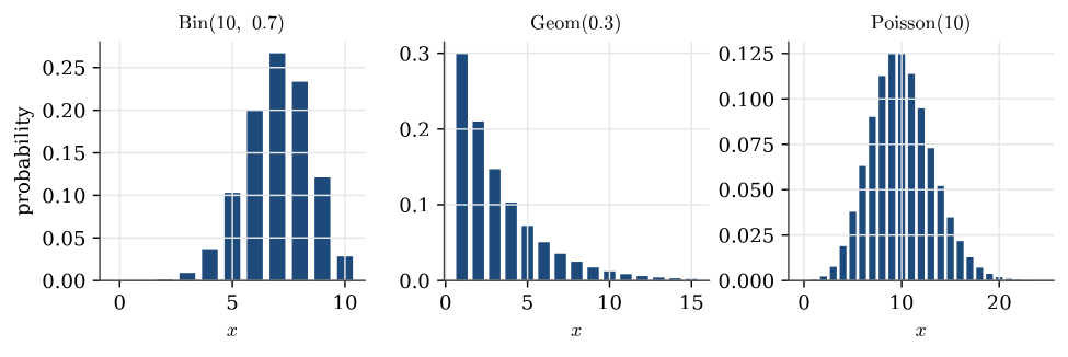
| Notation | x\sim\operatorname{Bin}(n,p) |
| Parameters | n\in\mathbb{Z}^{+}, p\in[0,1] |
| Support | x=0,1,\ldots,n |
| Mass function | p(x)=\binom{n}{x}p^{x}(1-p)^{n-x} |
| Mean | \mathbb{E}(x)=np |
| Variance | \operatorname{Var}(x)=np(1-p) |
| Conjugate prior | Beta distribution: p\sim\operatorname{Beta}(a,b), giving p\mid x\sim\operatorname{Beta}(a+x,b+n-x) |
| Taught in | Random variables and distributions |
| Part | Probability |
| Properties | 4 |
| Worked examples | 7 |
| Questions using it | 1 |
From the distribution sheet; mode and conjugate pairs from the formula lookup.
X has the binomial distribution with n trials and success probability p, written X\sim\operatorname{Bin}(n,p), when
\mathbb{P}(X=x)=\binom nx p^x(1-p)^{n-x},\qquad x=0,1,\ldots,n.
It is the number of successes in n independent \operatorname{Bern}(p) trials. Then \mathbb{E} X=np and \operatorname{Var}(X)=np(1-p).
Properties
Beta–Binomial conjugacy
Main article: Beta–Binomial conjugacy
\boxed{ \theta\mid x\sim \operatorname{Beta}(\alpha+x,\beta+n-x)}.
Beta–Binomial posterior prediction
Main article: Beta–Binomial posterior prediction
If \theta\mid x\sim\operatorname{Beta}(a,b) and, conditionally on \theta, \widetilde X\sim\operatorname{Bin}(m,\theta), then
\mathbb{P}(\widetilde X=k\mid x) =\binom mk\frac{B(k+a,m-k+b)}{B(a,b)}, \qquad k=0,\ldots,m.
For one future Bernoulli observation, \mathbb{P}(\widetilde Y=1\mid x)=a/(a+b).
Poisson limit of the binomial
Main article: Poisson limit of the binomial
If X_n\sim\operatorname{Bin}(n,p_n) with np_n\to\lambda as n\to\infty, then \mathbb{P}(X_n=x)\to e^{-\lambda}\lambda^x/x! for every x=0,1,2,\ldots
Central limit theorem
Main article: Central limit theorem
If the X_i are independent and identically distributed with mean \mu and variance \sigma^2\in(0,\infty), then for every x
\lim_{n\to\infty}\mathbb{P}\Bigl(\frac{S_n-n\mu}{\sigma\sqrt{n}}\le x\Bigr)=\Phi(x),
where \Phi is the standard normal distribution function.
Examples
Five future tosses
Worked example from The Beta–Binomial model
Suppose the prior is \theta\sim\operatorname{Beta}(2,2) and the observed data contain x=8 heads in n=10 tosses.
Question. Find the posterior predictive probability of a head on the next toss and the probability of at least four heads in five future tosses. Derive the predictive variance for the five-toss count and compare it with the variance obtained by plugging the posterior mean of \theta into a Binomial model.
Solution. The posterior calculation gives
\theta\mid x \sim\operatorname{Beta}(2+8,2+10-8) =\operatorname{Beta}(10,4).
For the very next toss, \begin{align*} \mathbb{P}(\widetilde Y=1\mid x) &=\mathbb{E}(\theta\mid x)\\ &=\frac{10}{10+4}\\ &=\frac57\\ &\approx0.714. \end{align*} The raw sample proportion is 8/10=0.8. The prediction is less extreme because it averages over the posterior produced by the data and the \operatorname{Beta}(2,2) prior.
Now let \widetilde X be the number of heads in m=5 future tosses. With a=10, b=4, and T=a+b=14, \mathbb{P}(\widetilde X=k\mid x) =\binom5k\frac{B(k+a,5-k+b)}{B(a,b)}, \qquad k=0,\ldots,5. For the rising factorial
(c)^{\overline r} =c(c+1)\cdots(c+r-1), \qquad (c)^{\overline 0}=1,
the Beta-function ratio satisfies
\frac{B(k+a,5-k+b)}{B(a,b)} =\frac{(a)^{\overline k}(b)^{\overline{5-k}}} {(a+b)^{\overline5}}.
Therefore the probability of at least four heads is \begin{align*} \mathbb{P}(\widetilde X\geq4\mid x) &=\mathbb{P}(\widetilde X=4\mid x) +\mathbb{P}(\widetilde X=5\mid x)\\ &=\frac{ \binom54(10)^{\overline4}(4)^{\overline1} +\binom55(10)^{\overline5}(4)^{\overline0}} {(14)^{\overline5}}\\ &=\frac{ 5(10\cdot11\cdot12\cdot13)(4) +(10\cdot11\cdot12\cdot13\cdot14)} {14\cdot15\cdot16\cdot17\cdot18}\\ &=\frac{583440}{1028160}\\ &\approx0.567. \end{align*}
This example also shows exactly why posterior prediction is more dispersed than a plug-in Binomial distribution. Conditional on \theta,
\mathbb{E}(\widetilde X\mid\theta)=5\theta, \qquad \operatorname{Var}(\widetilde X\mid\theta)=5\theta(1-\theta).
For \theta\mid x\sim\operatorname{Beta}(a,b) with T=a+b,
\mathbb{E}(\theta\mid x)=\frac aT, \qquad \operatorname{Var}(\theta\mid x)=\frac{ab}{T^2(T+1)}.
Moreover, \begin{align*} \mathbb{E}\{\theta(1-\theta)\mid x\} &=\mathbb{E}(\theta\mid x)-\mathbb{E}(\theta^2\mid x)\\ &=\frac aT-\frac{a(a+1)}{T(T+1)}\\ &=\frac{a(T+1)-a(a+1)}{T(T+1)}\\ &=\frac{a(T-a)}{T(T+1)}\\ &=\frac{ab}{T(T+1)}. \end{align*} Applying Equation (3) in Bayesian foundations, \begin{align*} \operatorname{Var}(\widetilde X\mid x) &=\mathbb{E}\{5\theta(1-\theta)\mid x\} +\operatorname{Var}(5\theta\mid x)\\ &=\frac{5ab}{T(T+1)} +\frac{25ab}{T^2(T+1)}\\ &=\frac{5ab(T+5)}{T^2(T+1)}\\ &=\frac{5(10)(4)(19)}{14^2(15)}\\ &=\frac{190}{147}\\ &\approx1.293. \end{align*} If one instead plugs in the posterior mean \widehat\theta=10/14, the variance would be only
5\widehat\theta(1-\widehat\theta) =5\left(\frac{10}{14}\right)\left(\frac4{14}\right) =\frac{50}{49} \approx1.020.
The difference is the second term in Equation (3) in Bayesian foundations: uncertainty about \theta.
Defective items in a box
Worked example from Random variables and distributions
Each item from a production line is defective with probability 0.05, independently of the others. A box holds 20 items.
Question. Find the expected number of defective items in a box, and the probability that a box has at most one.
Solution. The number of defectives is X\sim\operatorname{Bin}(20,0.05), so \mathbb{E} X=20\times0.05=1. Then
\mathbb{P}(X\le1)=0.95^{20}+20\times0.05\times0.95^{19}=0.358+0.377=0.736.
Although the average is exactly one defective, more than a quarter of boxes have two or more.
Normal approximation to a binomial
Worked example from Functions of random variables and limit theorems
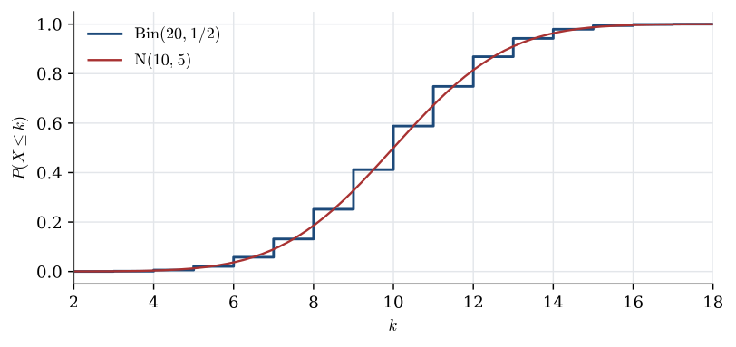
Let X\sim\operatorname{Bin}(20,1/2).
Question. Approximate \mathbb{P}(X\le8) by the central limit theorem, with and without a continuity correction, and compare with the exact value.
Solution. Here np=10 and np(1-p)=5. The exact probability is 0.2517. The plain approximation gives
\mathbb{P}(X\le8)\approx\Phi\Bigl(\frac{8-10}{\sqrt5}\Bigr)=\Phi(-0.894)=0.186,
which is poor. X is integer-valued, so \mathbb{P}(X\le8)=\mathbb{P}(X\le8.5), and the normal curve should be read at the midpoint between 8 and 9:
\mathbb{P}(X\le8)\approx\Phi\Bigl(\frac{8.5-10}{\sqrt5}\Bigr)=\Phi(-0.671)=0.251,
almost exact. A usual rule of thumb asks for both np and n(1-p) to be above 5.
Q6. Beta-Binomial conjugacy and prior influence
Question page: Q6. Beta-Binomial conjugacy and prior influence
Suppose X\mid\theta\sim\operatorname{Bin}(n,\theta), \qquad \theta\sim\operatorname{Beta}(a,b), where n\geq1, a,b>0, and the observed value of X is x.
(a) Derive the posterior density of \theta. Identify its distribution, parameters, and support. [3 marks]
(b) Express the posterior mean as a weighted average of the prior mean and x/n. Explain how the weight on the prior changes as n increases, with a and b fixed. [3 marks]
(c) Another statistician instead uses a prior uniform on (0,1/2). If x/n=4/5, can the posterior assign positive probability to \theta>1/2? Explain why or why not. [2 marks]
(d) Under squared-error loss, explain why the posterior mean is the Bayes estimate. Is it necessarily the Bayes estimate under a different loss? [2 marks]
Definitions. For a,b>0, a \operatorname{Beta}(a,b) density is \theta^{a-1}(1-\theta)^{b-1}/B(a,b) on (0,1), where B(a,b)=\int_0^1u^{a-1}(1-u)^{b-1}\,du. Here x is a Binomial success count out of known n. A Bayes estimate is an action d minimising posterior expected loss. Part (c) substitutes a restricted prior; part (d) returns to the Beta prior from (a).
(a) Posterior distribution
The likelihood and prior kernels are p(x\mid\theta)\propto\theta^x(1-\theta)^{n-x}, \qquad p(\theta)\propto\theta^{a-1}(1-\theta)^{b-1}. Therefore, \begin{aligned} p(\theta\mid x) &\propto p(x\mid\theta)p(\theta)\\ &\propto \theta^{a+x-1}(1-\theta)^{b+n-x-1}, \qquad 0<\theta<1. \end{aligned} Thus \boxed{ \theta\mid x\sim\operatorname{Beta}(a+x,b+n-x) }. The normalised posterior density is p(\theta\mid x) =\frac{\theta^{a+x-1}(1-\theta)^{b+n-x-1}} {B(a+x,b+n-x)}, \qquad 0<\theta<1.
(b) Posterior mean and prior influence
The posterior mean is \mathbb{E}(\theta\mid x)=\frac{a+x}{a+b+n}. Since the prior mean is \mathbb{E}(\theta)=a/(a+b), \begin{aligned} \mathbb{E}(\theta\mid x) &= \frac{a+b}{a+b+n}\frac{a}{a+b} +\frac{n}{a+b+n}\frac{x}{n}\\ &= \boxed{ \frac{a+b}{a+b+n}\mathbb{E}(\theta) +\frac{n}{a+b+n}\frac{x}{n} }. \end{aligned} The two weights sum to one. With a and b fixed, the prior weight (a+b)/(a+b+n) decreases to zero as n\to\infty, while the data weight increases to one.
(c) Restricted prior support
No. A prior uniform on (0,1/2) has density zero for \theta>1/2. Because p(\theta\mid x)\propto p(x\mid\theta)p(\theta), the posterior is also zero wherever the prior is zero. Hence \boxed{\mathbb{P}(\theta>1/2\mid x)=0}, even when x/n=4/5. The likelihood can reweight values inside the prior support, but it cannot create posterior mass outside that support.
(d) Bayes estimate under squared-error loss
Write m=\mathbb{E}(\theta\mid x) and expand \theta-d=(\theta-m)+(m-d). The cross term has posterior expectation 2(m-d)\mathbb{E}(\theta-m\mid x)=0. Consequently, for an estimate d, the posterior expected squared loss is \begin{aligned} \mathbb{E}\bigl[(\theta-d)^2\mid x\bigr] &= \operatorname{Var}(\theta\mid x) +\bigl\{\mathbb{E}(\theta\mid x)-d\bigr\}^2. \end{aligned} The variance term does not depend on d, so this expression is minimised by \boxed{ \widehat{\theta}_{\mathrm{Bayes}} =\mathbb{E}(\theta\mid x) =\frac{a+x}{a+b+n}. } The Bayes estimate depends on the loss function: for example, absolute-error loss gives a posterior median rather than necessarily the posterior mean.
Q44. Testing whether a coin is fair
Question page: Q44. Testing whether a coin is fair
[10 marks]
Suppose X\mid\theta\sim\operatorname{Binomial}(n,\theta). Compare M_0:\theta=\frac12, \qquad M_1:\theta\sim\operatorname{Beta}(a,b), with a,b>0 and equal prior model probabilities.
You may use B(a,b)=\int_0^1t^{a-1}(1-t)^{b-1}\,dt.
(a) Derive \mathbb{P}(X=x\mid M_0) and \mathbb{P}(X=x\mid M_1). [4 marks]
(b) Obtain the Bayes factor BF_{01} and the posterior probability \mathbb{P}(M_0\mid X=x). [3 marks]
(c) A student argues:
“Under a continuous Beta posterior, \mathbb{P}(\theta=1/2\mid x)=0, so Bayesian inference always rejects a fair coin.”
Explain the error. [3 marks]
Definitions. M_0 fixes \theta=1/2 and M_1 assigns a \operatorname{Beta}(a,b) prior, with a,b>0. Its density is \theta^{a-1}(1-\theta)^{b-1}/B(a,b), where B(a,b)=\int_0^1u^{a-1}(1-u)^{b-1}\,du. BF_{01} is the marginal-likelihood ratio favouring M_0. Prior model probabilities are equal; a model probability is distinct from a point probability within the continuous alternative.
(a) Marginal likelihoods. Under M_0, \theta=1/2 is fixed, so \boxed{\mathbb{P}(X=x\mid M_0)=\binom nx2^{-n}.} Under M_1, average the likelihood over the Beta prior: \begin{aligned} \mathbb{P}(X=x\mid M_1) &=\int_0^1\binom nx\theta^x(1-\theta)^{n-x} \frac{\theta^{a-1}(1-\theta)^{b-1}}{B(a,b)}\,d\theta\\ &=\frac{\binom nx}{B(a,b)} \int_0^1\theta^{a+x-1}(1-\theta)^{b+n-x-1}\,d\theta\\ &=\boxed{\binom nx\frac{B(a+x,b+n-x)}{B(a,b)}}. \end{aligned}
(b) Bayes factor and posterior model probability. The Bayes factor in favour of M_0 over M_1 is \boxed{ BF_{01} =\frac{\mathbb{P}(X=x\mid M_0)}{\mathbb{P}(X=x\mid M_1)} =2^{-n}\frac{B(a,b)}{B(a+x,b+n-x)}. } The binomial coefficients cancel in the ratio, but belong in the individual marginal likelihoods. Equal prior model probabilities give prior odds one, so posterior odds equal BF_{01}. Hence \boxed{ \mathbb{P}(M_0\mid X=x) =\frac{BF_{01}}{1+BF_{01}} =\frac{2^{-n}B(a,b)}{2^{-n}B(a,b)+B(a+x,b+n-x)}. }
(c) Error in the student’s argument. Under M_1 alone, \theta\mid x,M_1\sim\operatorname{Beta}(a+x,b+n-x), \qquad \mathbb{P}(\theta=1/2\mid x,M_1)=0, because this posterior is continuous. Every individual point has probability zero under it; that fact is not a test rejecting that particular value.
The model comparison instead assigns positive prior probability to the separate point-null model M_0. Both marginal likelihoods are positive for valid data, so \mathbb{P}(M_0\mid x)>0. In the combined model, \mathbb{P}(\theta=1/2\mid x)=\mathbb{P}(M_0\mid x), since M_0 places all its probability at 1/2 and M_1 contributes no point mass there. The student has confused a probability conditional on M_1 with the probability after allowing both models.
Twenty fair tosses
Question page: Twenty fair tosses
A fair coin is tossed 20 times.
Find the probability of exactly 10 heads.
Find the probability of 15 or more heads.
The number of heads is \operatorname{Bin}(20,1/2).
\binom{20}{10}/2^{20}\approx 0.176.
\sum_{k=15}^{20}\binom{20}{k}/2^{20}\approx 0.0207.
Ten voters
Question page: Ten voters
In a large population, 40% vote for candidate A. Ten people are drawn independently. Find the probability that exactly four of them vote for A.
The number who vote for A is \operatorname{Bin}(10,0.4), so the probability of exactly four is \binom{10}{4}(0.4)^4(0.6)^6.
Figures
Used in
- Taught in Random variables and distributions, where the derivation and examples are.
- Also used in Random experiments and probability · Simulation · Reliability · The Beta–Binomial model · Categorical data and the Dirichlet distribution
- Questions that use it (1) — Counting degrees of freedom
- All 27 questions on Random variables and distributions
See also
Categorical and multinomial models · Random variable · Cumulative distribution function · Discrete distribution · Continuous distribution · Expectation · Expectation of a function · Variance