Normal distribution
Definition taught in Random variables and distributions, part of Probability · Also on the distribution sheet
Normal distribution
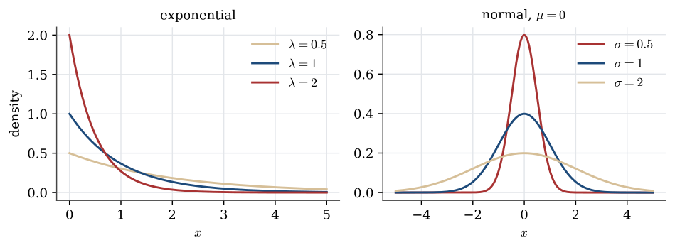
| Notation | X\sim\operatorname{N}(\mu,\sigma^{2}) |
| Parameters | \mu\in\mathbb{R}, \sigma>0 |
| Support | x\in\mathbb{R} |
| Density | p(x)=\frac{1}{\sqrt{2\pi}\,\sigma}\exp\Bigl(-\frac{(x-\mu)^{2}}{2\sigma^{2}}\Bigr) |
| Mean | \mathbb{E}(X)=\mu |
| Variance | \operatorname{Var}(X)=\sigma^{2} |
| Conjugate prior for | X_i\mid\mu\sim\operatorname{N}(\mu,\sigma^2) with prior \mu\sim\operatorname{N}(\mu_0,\sigma_0^2), giving Equation (2) in Conjugate analysis for normal models |
| Conjugate prior | Inverse-Gamma distribution: \sigma^2\sim\operatorname{InvGamma}(a,b), giving \operatorname{InvGamma}(a+n/2,b+S_\mu/2) |
| Taught in | Random variables and distributions |
| Part | Probability |
| Properties | 5 |
| Worked examples | 5 |
| Questions using it | 10 |
From the distribution sheet; mode and conjugate pairs from the formula lookup.
X has the normal distribution with mean \mu and variance \sigma^2>0, written X\sim\operatorname{N}(\mu,\sigma^2), when its density is
\frac1{\sigma\sqrt{2\pi}}\exp\Bigl\{-\frac{(x-\mu)^2}{2\sigma^2}\Bigr\},\qquad x\in\mathbb{R}.
The standard normal distribution is \operatorname{N}(0,1), with distribution function written \Phi.
Properties
Normal–Normal conjugacy
Main article: Normal–Normal conjugacy
\boxed{ \mu\mid{\boldsymbol{x}}\sim\operatorname{N}(\mu_1,\sigma_1^2)}, with \begin{aligned} \sigma_1^2 &=\frac1A =\left(\frac n{\sigma^2}+\frac1{\sigma_0^2}\right)^{-1} =\frac{\sigma^2\sigma_0^2}{n\sigma_0^2+\sigma^2}, \\ \mu_1 &=\frac BA =\frac{\sum_i x_i/\sigma^2+\mu_0/\sigma_0^2} {n/\sigma^2+1/\sigma_0^2}\\ &=\frac{n\overline x\,\sigma_0^2+\mu_0\sigma^2} {n\sigma_0^2+\sigma^2}. \end{aligned}
Normal–inverse-Gamma variance update
Main article: Normal–inverse-Gamma variance update
\boxed{ \sigma^2\mid{\boldsymbol{x}} \sim\operatorname{InvGamma}\!\left( \alpha_0+\frac n2, \beta_0+\frac12S_\mu \right)}.
Full conditionals under independent priors
Main article: Full conditionals under independent priors
Holding \sigma^2 fixed, the calculation from Equation (1) in Conjugate analysis for normal models applies verbatim: \boxed{ \mu\mid\sigma^2,{\boldsymbol{x}} \sim\operatorname{N}\!\left( \frac{n\overline x\,\sigma_0^2+\mu_0\sigma^2} {n\sigma_0^2+\sigma^2}, \frac{\sigma^2\sigma_0^2}{n\sigma_0^2+\sigma^2} \right)}. Holding \mu fixed, the calculation from Equation (3) in Conjugate analysis for normal models applies: \boxed{ \sigma^2\mid\mu,{\boldsymbol{x}} \sim\operatorname{InvGamma}\!\left( \alpha_0+\frac n2, \beta_0+\frac12\sum_{i=1}^n(x_i-\mu)^2 \right)}.
Precision weighting
Main article: Precision weighting
Writing
w=\frac{\sigma^2}{n\sigma_0^2+\sigma^2}
turns Equation (2) in Conjugate analysis for normal models into
\mu_1=(1-w)\overline x+w\mu_0.
The posterior mean is therefore a precision-weighted average. Equivalently, if \kappa_0=\sigma^2/\sigma_0^2, then
\mu_1=\frac{n\overline x+\kappa_0\mu_0}{n+\kappa_0}.
Thus the prior behaves like \kappa_0 observations whose mean is \mu_0. In the special case \sigma_0^2=\sigma^2, it behaves like one extra observation at \mu_0.
Normal sample theorem
Main article: Normal sample theorem
If X_1,\ldots,X_n are a random sample from \operatorname{N}(\mu,\sigma^2), then
- \overline X is \operatorname{N}(\mu,\sigma^2/n),
- (n-1)s^2/\sigma^2 is \chi^2_{n-1}, and
- \overline X and s^2 are independent.
Examples
IQ scores
Worked example from Random variables and distributions
Suppose IQ scores are \operatorname{N}(100,16^2).
Question. What fraction of people score between 90 and 110, and what fraction above 130?
Solution. Standardise: (90-100)/16=-0.625 and (110-100)/16=0.625, so
\mathbb{P}(90<X\le110)=\Phi(0.625)-\Phi(-0.625)=2\Phi(0.625)-1=0.468.
Above 130, z=1.875 and \mathbb{P}(X>130)=1-\Phi(1.875)=0.030, about one person in 33. These are the class probabilities used to sort recruits in Chi-squared tests.
Q7. Normal estimation and prediction
Question page: Q7. Normal estimation and prediction
Suppose that, conditionally on \mu, X_1,\ldots,X_n\mid\mu \overset{\mathrm{iid}}{\sim}\mathcal{N}(\mu,\sigma^2), where \sigma^2>0 is known. Use the prior \mu\sim\mathcal{N}(\mu_0,\tau^2), where \tau^2>0 is known.
(a) By completing the square in \mu, derive its posterior distribution. Denote the posterior mean and variance by m and v. [4 marks]
(b) Let X_{\mathrm{new}} be a further observation, independent of the observed sample given \mu. Derive its posterior predictive distribution. Explain the two sources of its variance. [4 marks]
(c) As n\to\infty, with \sigma^2 and the prior fixed, what happens to the posterior variance of \mu and the predictive variance of X_{\mathrm{new}}? Explain why they behave differently. [2 marks]
Definitions. The notation N(m,v) uses mean m and variance v; precision is 1/v. The data have known variance \sigma^2>0, and the mean prior is N(\mu_0,\tau^2) with \tau^2>0. Write \bar x=n^{-1}\sum_i x_i. Posterior prediction averages a new observation’s sampling distribution over the parameter posterior; that observation is independent of the original sample conditional on \mu.
(a) Posterior distribution of \mu
Start from independence and the specified prior: L(\mu;{\boldsymbol{x}})=(2\pi\sigma^2)^{-n/2} \exp\left[-\frac{\sum_i(x_i-\mu)^2}{2\sigma^2}\right], \qquad p(\mu)\propto\exp\left[-\frac{(\mu-\mu_0)^2}{2\tau^2}\right]. The identity \sum_i(x_i-\mu)^2=\sum_i(x_i-\bar x)^2+n(\mu-\bar x)^2 follows by expanding around \bar x; the cross term is zero because \sum_i(x_i-\bar x)=0. Bayes’ theorem multiplies these two kernels. Ignoring terms that do not depend on \mu, \begin{aligned} p(\mu\mid{\boldsymbol{x}}) &\propto \exp\left[ -\frac{n}{2\sigma^2}(\mu-\bar{x})^2 -\frac{1}{2\tau^2}(\mu-\mu_0)^2 \right]\\ &\propto \exp\left[ -\frac12 \left\{ \left(\frac{n}{\sigma^2}+\frac{1}{\tau^2}\right)\mu^2 -2\left( \frac{n\bar{x}}{\sigma^2}+\frac{\mu_0}{\tau^2} \right)\mu \right\} \right]. \end{aligned} Define v=\left(\frac{n}{\sigma^2}+\frac{1}{\tau^2}\right)^{-1}, \qquad m=v\left( \frac{n\bar{x}}{\sigma^2}+\frac{\mu_0}{\tau^2} \right). Completing the square gives p(\mu\mid{\boldsymbol{x}}) \propto \exp\left[-\frac{(\mu-m)^2}{2v}\right], so \boxed{\mu\mid{\boldsymbol{x}}\sim\mathcal{N}(m,v)}. Equivalently, v=\frac{\sigma^2\tau^2}{n\tau^2+\sigma^2}, \qquad m=\frac{n\tau^2\bar{x}+\sigma^2\mu_0} {n\tau^2+\sigma^2}.
(b) Posterior predictive distribution
Conditional on \mu, X_{\mathrm{new}}=\mu+\varepsilon, \qquad \varepsilon\sim\mathcal{N}(0,\sigma^2), where \varepsilon is independent of \mu\mid{\boldsymbol{x}}. Since \mu\mid{\boldsymbol{x}}\sim\mathcal{N}(m,v), \boxed{ X_{\mathrm{new}}\mid{\boldsymbol{x}} \sim\mathcal{N}(m,\sigma^2+v) }. The predictive variance can also be obtained from \begin{aligned} \operatorname{Var}(X_{\mathrm{new}}\mid{\boldsymbol{x}}) &= \mathbb{E}\!\left[ \operatorname{Var}(X_{\mathrm{new}}\mid\mu,{\boldsymbol{x}}) \mid{\boldsymbol{x}} \right]\\ &\quad+ \operatorname{Var}\!\left( \mathbb{E}[X_{\mathrm{new}}\mid\mu,{\boldsymbol{x}}] \mid{\boldsymbol{x}} \right)\\ &=\sigma^2+v. \end{aligned} Here \sigma^2 is future-observation noise and v is uncertainty about the unknown mean.
(c) Limiting variances
As n\to\infty, v=\left(\frac{n}{\sigma^2}+\frac{1}{\tau^2}\right)^{-1} \longrightarrow0, whereas \operatorname{Var}(X_{\mathrm{new}}\mid{\boldsymbol{x}}) =\sigma^2+v \longrightarrow\sigma^2. Increasing n removes uncertainty about \mu, but it does not remove the irreducible sampling variation in a new observation.
Question 1. Normal mean, known variance
Question page: Question 1. Normal mean, known variance
Let
X_i\mid\mu\stackrel{\mathrm{iid}}{\sim}\operatorname{N}(\mu,\sigma^2),
with \sigma^2 known and \mu\sim \operatorname{N}(\mu_0,\sigma_0^2).
(a) Using only the precision-addition rule and the precision-weighted mean, write the two updated parameters of the posterior for \mu.
(b) Define the prior equivalent sample size, and state what it counts.
(c) Explain why the posterior mean is a precision-weighted average of the prior mean and the sample mean.
(d) State and interpret the limiting posterior mean and variance as n\to\infty, with the prior parameters fixed and \bar X_n\to\mu^{\ast}.
(e) State the posterior predictive distribution of one new observation X_{\mathrm{new}}, conditionally independent of the sample given \mu.
(f) Explain why the posterior predictive variance is larger than the posterior variance of \mu.
Definitions. Write \bar x=n^{-1}\sum_i x_i. A normal distribution \operatorname{N}(m,v) has mean m and variance v; its precision is 1/v. Here \sigma^2 is the known observation variance, \sigma_0^2 is the prior variance of the unknown mean, and \sigma_1^2 will be its posterior variance. These are variances of different objects.
(a) The data precision of n observations is n/\sigma^2, and the prior precision is 1/\sigma_0^2. Precision addition gives
\frac1{\sigma_1^2} = \frac n{\sigma^2}+\frac1{\sigma_0^2}.
The posterior mean is the precision-weighted average of \bar x and \mu_0:
\mu_1 = \frac{(n/\sigma^2)\bar x+(1/\sigma_0^2)\mu_0}{n/\sigma^2+1/\sigma_0^2} = \frac{n\bar x\,\sigma_0^2+\mu_0\sigma^2}{n\sigma_0^2+\sigma^2}.
\boxed{\mu\mid x\sim \operatorname{N}(\mu_1,\sigma_1^2).}
(b)
\kappa_0=\frac{\sigma^2}{\sigma_0^2}.
It counts how many observations of variance \sigma^2 have the same precision as the prior, since 1/\sigma_0^2=\kappa_0/\sigma^2.
Consequently, \mu_1=(n\bar x+\kappa_0\mu_0)/(n+\kappa_0) and \sigma_1^2=\sigma^2/(n+\kappa_0). The equivalent sample size measures information about the common mean. It need not be an integer or represent actual previous observations.
(c) Up to an additive constant free of \mu, the log posterior is
-\frac{n}{2\sigma^2}(\bar x-\mu)^2-\frac{1}{2\sigma_0^2}(\mu-\mu_0)^2.
Its derivative is (n/\sigma^2)(\bar x-\mu)-(1/\sigma_0^2)(\mu-\mu_0). Setting the derivative equal to zero balances the two pulls, so
\mu_1 = \frac{(n/\sigma^2)\bar x+(1/\sigma_0^2)\mu_0}{n/\sigma^2+1/\sigma_0^2}.
The second derivative is -n/\sigma^2-1/\sigma_0^2<0, so this stationary point is the unique posterior mode. The posterior is normal, hence its mode equals its mean. This derives the weighting rule: moving away from a more precise source incurs a larger quadratic penalty. The two weights are nonnegative and sum to one, so the posterior mean lies between \bar x and \mu_0.
(d) Let w_n=(n/\sigma^2)/(n/\sigma^2+1/\sigma_0^2). Then w_n\to 1 and
\mu_1=w_n\bar X_n+(1-w_n)\mu_0\to\mu^{\ast}, \qquad \sigma_1^2=\Bigl(\frac n{\sigma^2}+\frac1{\sigma_0^2}\Bigr)^{-1}\to 0.
With the prior held fixed, the data precision dominates. The posterior concentrates at the limiting sample mean.
This conclusion uses the stated convergence \bar X_n\to\mu^\ast. Under the iid normal model with true mean \mu^\ast, that convergence follows from the law of large numbers. A fixed prior contributes a fixed amount of precision, while the likelihood contributes an amount growing linearly with n.
(e) Given \mu, X_{\mathrm{new}} is independent of the sample and X_{\mathrm{new}}\mid\mu\sim \operatorname{N}(\mu,\sigma^2). Since \mu\mid{\boldsymbol{x}}\sim \operatorname{N}(\mu_1,\sigma_1^2),
\boxed{X_{\mathrm{new}}\mid{\boldsymbol{x}}\sim \operatorname{N}(\mu_1,\sigma^2+\sigma_1^2).}
To see the distributional result, write X_{\mathrm{new}}=\mu+\varepsilon_{\mathrm{new}}, where \varepsilon_{\mathrm{new}}\sim\operatorname{N}(0,\sigma^2) is independent of the posterior draw of \mu. Conditional on the observed sample, this is a sum of two independent normal variables. Merely replacing \mu by \mu_1 would omit uncertainty about the unknown mean.
(f) By the law of total variance,
\operatorname{Var}(X_{\mathrm{new}}\mid{\boldsymbol{x}}) = \mathbb{E}[\sigma^2\mid{\boldsymbol{x}}]+\operatorname{Var}(\mu\mid{\boldsymbol{x}}) = \sigma^2+\sigma_1^2.
The term \sigma_1^2 is uncertainty about \mu. The term \sigma^2 is the variance of a new observation even if \mu is known. Both are positive, so the predictive variance exceeds the posterior variance of \mu.
Two standard normal probabilities
Question page: Two standard normal probabilities
Let X be standard normal. Using \Phi(1.3)\approx 0.9032 and \Phi(1.4)\approx 0.9192, evaluate \mathbb{P}(X\le 1.4) and \mathbb{P}(X>-1.3).
\mathbb{P}(X\le 1.4)=\Phi(1.4)\approx 0.9192. The standard normal density is symmetric, so \mathbb{P}(X>-1.3)=\mathbb{P}(X<1.3)=\Phi(1.3)\approx 0.9032.
Probabilities for a shifted normal
Question page: Probabilities for a shifted normal
Let Y\sim\operatorname{N}(1,4). Using \Phi(0.5)\approx 0.6915 and \Phi(1)\approx 0.8413, evaluate \mathbb{P}(Y\le 3) and \mathbb{P}(-1\le Y\le 2).
Write Y=1+2X with X standard normal. Then \mathbb{P}(Y\le 3)=\mathbb{P}(X\le 1)=\Phi(1)\approx 0.8413, and
\mathbb{P}(-1\le Y\le 2)=\mathbb{P}(-1\le X\le 1/2)=\Phi(1/2)-(1-\Phi(1))\approx 0.6915-0.1587=0.5328.
Used in
- Taught in Random variables and distributions, where the derivation and examples are.
- Also used in Functions of random variables and limit theorems · Linear regression · Descriptive statistics · Bayesian linear regression · Introduction to generalised linear models · Probability-integral residuals · Random slopes, and a binary mixed model
- Questions that use it (10) — Rescaling a standard normal draw · State the probability functions · Counting degrees of freedom · Q25 (answer) · Q45 (answer) · Question 1 (answer) · Question 4 · Question 5 (answer) · Question 20 (answer) · Question 21 (answer)
- All 27 questions on Random variables and distributions
See also
Cumulative distribution function · Normal quantile plot · Studentised coefficient pivot · Random variable · Discrete distribution · Continuous distribution · Expectation · Expectation of a function