Poisson distribution
Definition taught in Random variables and distributions, part of Probability · Also on the distribution sheet
Poisson distribution
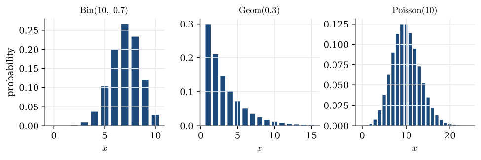
| Notation | x\sim\operatorname{Poisson}(\theta) |
| Parameters | \theta>0 |
| Support | x=0,1,2,\ldots |
| Mass function | p(x)=e^{-\theta}\theta^{x}/x! |
| Mean | \mathbb{E}(x)=\theta |
| Variance | \operatorname{Var}(x)=\theta |
| Conjugate prior | Gamma distribution: \theta\sim\operatorname{Gamma}(a,b), giving \operatorname{Gamma}(a+\sum_i x_i,b+n) |
| Taught in | Random variables and distributions |
| Part | Probability |
| Properties | 2 |
| Worked examples | 6 |
| Questions using it | 1 |
From the distribution sheet; mode and conjugate pairs from the formula lookup.
X has the Poisson distribution with mean \lambda>0, written X\sim\operatorname{Poisson}(\lambda), when
\mathbb{P}(X=x)=e^{-\lambda}\frac{\lambda^x}{x!},\qquad x=0,1,2,\ldots
Then \mathbb{E} X=\operatorname{Var}(X)=\lambda.
Properties
Generic exponential-family conjugate update
Main article: Generic exponential-family conjugate update
The hyperparameters update as \boxed{ \alpha\leftarrow \alpha+S({\boldsymbol{x}}), \qquad \beta\leftarrow\beta+n.}
Poisson limit of the binomial
Main article: Poisson limit of the binomial
If X_n\sim\operatorname{Bin}(n,p_n) with np_n\to\lambda as n\to\infty, then \mathbb{P}(X_n=x)\to e^{-\lambda}\lambda^x/x! for every x=0,1,2,\ldots
Examples
Poisson natural form and Gamma conjugacy
Worked example from Exponential families and conjugacy
Question. For iid Poisson observations with mean \theta, write the model in the a(\theta), b(x), c(\theta), T(x) form, identify the sufficient statistic, and derive the corresponding conjugate prior and posterior update.
Solution. For one Poisson observation, \begin{align*} p(x\mid\theta) &=\frac{e^{-\theta}\theta^x}{x!}\\ &=\frac1{x!}\exp\{x\log\theta\}e^{-\theta}\\ &=\frac{b(x)\exp\{c(\theta)T(x)\}}{a(\theta)}, \end{align*} with
b(x)=\frac1{x!}, \qquad c(\theta)=\log\theta, \qquad T(x)=x, \qquad a(\theta)=e^\theta.
For the Poisson model, the definition Equation (4) in Exponential families and conjugacy gives S({\boldsymbol{x}})=\sum_i x_i. The joint likelihood is \begin{align*} p({\boldsymbol{x}}\mid\theta) &=\prod_{i=1}^n\frac{e^{-\theta}\theta^{x_i}}{x_i!}\\ &=\left(\prod_{i=1}^n\frac1{x_i!}\right) \exp\{(\log\theta)S({\boldsymbol{x}})-n\theta\}. \end{align*} The factorisation theorem shows that S({\boldsymbol{X}}) is sufficient for \theta. It is also minimal sufficient by the likelihood-ratio criterion. Because the natural parameter c(\theta)=\log\theta ranges over the open set \mathbb{R}, S({\boldsymbol{X}}) is complete as well.
The generic prior Equation (6) in Exponential families and conjugacy becomes \begin{align*} p(\theta\mid\alpha,\beta) &\propto \frac{\exp\{\alpha\log\theta\}}{(e^\theta)^\beta}\\ &=\theta^\alpha e^{-\beta\theta}. \end{align*} This is the kernel of \operatorname{Gamma}(\alpha+1,\beta), not \operatorname{Gamma}(\alpha,\beta). Using the sufficient statistic S({\boldsymbol{x}}), \begin{align*} p(\theta\mid{\boldsymbol{x}}) &\propto \theta^{S({\boldsymbol{x}})} e^{-n\theta}\theta^\alpha e^{-\beta\theta}\\ &=\theta^{S({\boldsymbol{x}})+\alpha}e^{-(n+\beta)\theta}, \end{align*} so \boxed{ \theta\mid{\boldsymbol{x}} \sim\operatorname{Gamma}(\alpha+S({\boldsymbol{x}})+1,\beta+n)}. Its posterior mean is \begin{align*} \mathbb{E}(\theta\mid{\boldsymbol{x}}) &=\frac{\alpha+S({\boldsymbol{x}})+1}{\beta+n}\\ &=\frac{(\alpha+1)+n\overline x}{\beta+n}\\ &=\frac\beta{\beta+n}\frac{\alpha+1}{\beta} +\frac n{\beta+n}\overline x. \end{align*} The prior therefore behaves, for the mean, as \beta prior observations with total count \alpha+1.
Houses on a village grid
Worked example from Chi-squared tests
A village of 12 square kilometres is divided into 1200 plots, and the 911 houses are counted plot by plot. If houses are placed at random, the count on a plot should be Poisson.
| Houses on a plot | 0 | 1 | 2 | 3 | 4 | 5 | 6 | 7 | 8 | 9 |
|---|---|---|---|---|---|---|---|---|---|---|
| Plots | 584 | 398 | 168 | 35 | 9 | 4 | 0 | 1 | 0 | 1 |
Question. Test whether the counts per plot are Poisson.
Solution. The maximum likelihood estimate of the Poisson mean is the average count, \widehat\mu=911/1200=0.7592. The fitted expected number of plots with i houses is 1200\,e^{-\widehat\mu}\widehat\mu^{\,i}/i!: 561.67, 426.40, 161.85 and 40.96 for 0 to 3 houses, then 7.77, 1.18 and less than 0.2 after that. To keep every expectation at least 5, merge 4 or more houses into one class, with observed count 15 and expected count 9.12. With k=5 classes and r=1 estimated parameter,
T=\frac{(584-561.67)^2}{561.67}+\frac{(398-426.40)^2}{426.40}+\frac{(168-161.85)^2}{161.85}+\frac{(35-40.96)^2}{40.96}+\frac{(15-9.12)^2}{9.12}=7.67
on 5-1-1=3 degrees of freedom. Since \chi^2_{3;0.95}=7.815, the test just fails to reject at the 5% level; the p-value is 0.053. Most of the statistic comes from the merged tail class: there are more crowded plots, and fewer plots with a single house, than a Poisson law allows. The evidence that houses are not placed at random is suggestive, not conclusive.
A rare fault
Worked example from Random variables and distributions
A machine makes 1000 parts a day, and each part has a fault with probability 0.002, independently.
Question. Find the probability that a day has at most one faulty part, exactly and by the Poisson approximation.
Solution. The exact count is \operatorname{Bin}(1000,0.002), and \mathbb{P}(X\le1)=0.998^{1000}+1000\times0.002\times0.998^{999}=0.4057. The Poisson approximation uses \lambda=1000\times0.002=2:
\mathbb{P}(X\le1)\approx e^{-2}(1+2)=0.4060.
The two agree to three decimal places. The approximation is good whenever n is large and p is small, and it needs only the product np.
Q53. Poisson flaws and posterior odds
Question page: Q53. Poisson flaws and posterior odds
[12 marks]
A textile manufacturer counts flaws in equal-length rolls of fabric. Assume X_i\mid\theta\overset{\mathrm{iid}}{\sim}\operatorname{Poisson}(\theta), \qquad i=1,\ldots,10, where \theta is the mean number of flaws per roll.
Ten inspected rolls contain 32 flaws in total. The prior is \theta\sim\operatorname{Gamma}(8,2), using the shape–rate convention: \pi(\theta)=\frac{2^8}{\Gamma(8)}\theta^7e^{-2\theta}, \qquad\theta>0. The manufacturer considers the process acceptable if \theta\le4.
(a) Form the likelihood and derive the posterior distribution of \theta. [4 marks]
(b) Find the posterior mean. Show that it lies between the prior mean and the observed sample mean. [2 marks]
(c) Define H_0:\theta\le4,\qquad H_1:\theta>4. Write an integral for \mathbb P(H_0\mid{\boldsymbol{x}}), including the normalising constant. Hence express the posterior odds in favour of H_0. You do not need to evaluate the integral. [3 marks]
(d) A colleague argues:
“The posterior mean is below 4, so the probability that the process is acceptable must be 1.”
Explain why this is incorrect. Would changing H_0 to \theta<4 change its posterior probability? Justify your answer. [3 marks]
Definitions. For Gamma shape–rate parameters (A,B), the density is B^A\theta^{A-1}e^{-B\theta}/\Gamma(A) on \theta>0 and the mean is A/B. Here n=10, \sum_i x_i=32, and the prior is \operatorname{Gamma}(8,2). Write q=\mathbb P(\theta\le4\mid{\boldsymbol{x}}). Posterior odds in favour of this event over its complement are q/(1-q).
(a) Likelihood and posterior. Conditional independence gives, for observed nonnegative integer counts, \begin{aligned} L(\theta;{\boldsymbol{x}}) &=\prod_{i=1}^{10}\frac{e^{-\theta}\theta^{x_i}}{x_i!} =\frac{\theta^{\sum_i x_i}e^{-10\theta}}{\prod_{i=1}^{10}x_i!}\\ &\propto\theta^{32}e^{-10\theta},\qquad\theta>0. \end{aligned} The factorial term does not depend on \theta, so only the total count is needed for this likelihood kernel. Multiplying by the prior kernel, \begin{aligned} \pi(\theta\mid{\boldsymbol{x}}) &\propto L(\theta;{\boldsymbol{x}})\pi(\theta)\\ &\propto\theta^{32}e^{-10\theta}\theta^7e^{-2\theta} =\theta^{39}e^{-12\theta}. \end{aligned} Matching \theta^{A-1}e^{-B\theta} gives A=40 and B=12. Thus \boxed{\theta\mid{\boldsymbol{x}}\sim\operatorname{Gamma}(40,12) \quad\text{(shape--rate)},\qquad\theta>0,} with normalised posterior density \boxed{\pi(\theta\mid{\boldsymbol{x}}) =\frac{12^{40}}{\Gamma(40)}\theta^{39}e^{-12\theta}, \qquad\theta>0.}
(b) Posterior mean and shrinkage. The prior mean, sample mean, and posterior mean are respectively \mathbb{E}[\theta]=\frac82=4,\qquad \bar x=\frac{32}{10}=3.2,\qquad \boxed{\mathbb{E}[\theta\mid{\boldsymbol{x}}]=\frac{40}{12}=\frac{10}{3}.} In particular, 3.2<10/3<4. More explicitly, \mathbb{E}[\theta\mid{\boldsymbol{x}}] =\frac{8+32}{2+10} =\frac{2}{12}\left(\frac82\right) +\frac{10}{12}\left(\frac{32}{10}\right) =\frac16\mathbb{E}[\theta]+\frac56\bar x. The weights are positive and sum to one, so the posterior mean lies strictly between the two distinct means.
(c) Posterior probability and odds. Let q=\mathbb P(H_0\mid{\boldsymbol{x}}). Integrating the normalised posterior density over the acceptable region gives \boxed{q=\mathbb P(\theta\le4\mid{\boldsymbol{x}}) =\frac{12^{40}}{\Gamma(40)} \int_0^4\theta^{39}e^{-12\theta}\,d\theta.} The two hypotheses exhaust the parameter space, so \mathbb P(H_1\mid{\boldsymbol{x}})=1-q. Therefore the posterior odds in favour of H_0 are q:(1-q), or, as a ratio, \boxed{ \frac{\mathbb P(H_0\mid{\boldsymbol{x}})}{\mathbb P(H_1\mid{\boldsymbol{x}})} =\frac{q}{1-q} =\frac{\displaystyle\int_0^4\theta^{39}e^{-12\theta}\,d\theta} {\displaystyle\int_4^\infty\theta^{39}e^{-12\theta}\,d\theta}. } The common normalising constant cancels in the odds ratio, but it is required in the probability integral above. No numerical evaluation is needed.
(d) A mean below the threshold does not imply certainty. The posterior mean is an average of possible values of \theta, not an upper bound on them. Although \mathbb{E}[\theta\mid{\boldsymbol{x}}]=10/3<4, the \operatorname{Gamma}(40,12) density is strictly positive for every \theta>0, including values above 4. Consequently, \mathbb P(\theta>4\mid{\boldsymbol{x}}) =\frac{12^{40}}{\Gamma(40)} \int_4^\infty\theta^{39}e^{-12\theta}\,d\theta>0, so \mathbb P(\theta\le4\mid{\boldsymbol{x}})<1. A point estimate below the threshold does not eliminate posterior uncertainty about acceptability.
Replacing \theta\le4 by \theta<4 does not change the posterior probability. The posterior is continuous, and hence \mathbb P(\theta=4\mid{\boldsymbol{x}})=0. Therefore \boxed{\mathbb P(\theta<4\mid{\boldsymbol{x}}) =\mathbb P(\theta\le4\mid{\boldsymbol{x}}).}
Key result. The posterior mean answers “what is the posterior average of \theta?” The posterior probability of H_0 answers “how much posterior probability lies at or below 4?” These are different summaries.
Q32. Deriving the Poisson log-likelihood
Question page: Q32. Deriving the Poisson log-likelihood
[3 marks]
Suppose, conditional on fixed covariates, Y_i\mid\mathbf X_i \overset{\mathrm{ind}}{\sim}\operatorname{Poisson}(\mu_i), \qquad \mu_i=\exp(\mathbf X_i^\top\boldsymbol\beta). Starting from the Poisson probability mass function, show that \ell(\boldsymbol\beta) =\sum_{i=1}^{n}\left[ Y_i\mathbf X_i^\top\boldsymbol\beta -\exp(\mathbf X_i^\top\boldsymbol\beta) \right]+C. State exactly what C contains and why it can be ignored when maximising over \boldsymbol\beta.
Definitions. Let \mathbf X_i be a fixed column vector of predictors and X the matrix with rows \mathbf X_i^\top. Write \eta_i=\mathbf X_i^\top\boldsymbol\beta and \mu_i=e^{\eta_i}. The likelihood is the joint Poisson mass function evaluated at observed counts \mathbf y, and \ell=\log L. An additive constant may depend on the data but not on the parameter \boldsymbol\beta being maximised over.
For observed counts y_i\in\{0,1,2,\ldots\}, \mathbb{P}(Y_i=y_i\mid\mathbf X_i) =\frac{e^{-\mu_i}\mu_i^{y_i}}{y_i!}, \qquad \mu_i=\exp(\mathbf X_i^\top\boldsymbol\beta). Conditional independence gives L(\boldsymbol\beta;\mathbf y,X) =\prod_{i=1}^n\frac{e^{-\mu_i}\mu_i^{y_i}}{y_i!}. Taking logarithms, \ell(\boldsymbol\beta) =\sum_{i=1}^n\{-\mu_i+y_i\log\mu_i-\log(y_i!)\}. Since \log\mu_i=\mathbf X_i^\top\boldsymbol\beta, this becomes \boxed{ \ell(\boldsymbol\beta) =\sum_{i=1}^n \left[y_i\mathbf X_i^\top\boldsymbol\beta -\exp(\mathbf X_i^\top\boldsymbol\beta)\right]+C, \quad C=-\sum_{i=1}^n\log(y_i!). } The constant C depends only on the observed responses, not on \boldsymbol\beta. Therefore adding or removing it does not change the maximiser over \boldsymbol\beta, and its derivatives with respect to \boldsymbol\beta are zero. Writing Y_i instead of y_i gives the random-data version in the question.
Key result. “Constant” means constant with respect to the parameter being optimised, not necessarily independent of the data.
Particles in an hour
Question page: Particles in an hour
A source emits a particle in a given second with probability 1/100, independently across seconds. Let X be the number of particles emitted in one hour of 3600 seconds. Give the Poisson parameter that approximates the distribution of X.
The exact count is \operatorname{Bin}(3600,1/100). The Poisson approximation has mean 3600/100=36.
Used in
- Taught in Random variables and distributions, where the derivation and examples are.
- Also used in Standard errors, and models for counts · Paired comparisons, and how far a fit is from the data · Marginal models, and two responses at once
- Questions that use it (1) — State the probability functions
- All 27 questions on Random variables and distributions
See also
Random variable · Cumulative distribution function · Discrete distribution · Continuous distribution · Expectation · Expectation of a function · Variance · Probability generating function