Least-squares line
Definition taught in Linear regression, part of Statistical inference
Least-squares line
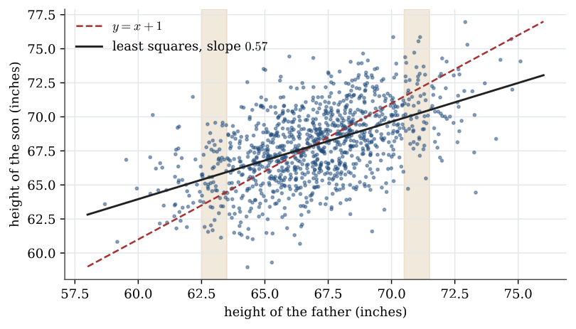
| Type | Definition |
| Taught in | Linear regression |
| Part | Statistical inference |
| Properties | 1 |
| Worked examples | 4 |
| Questions using it | 1 |
For points (x_1,y_1),\ldots,(x_n,y_n) with the x_i not all equal, the least-squares line y=b_0+b_1x minimises
L(b_0,b_1)=\sum_{i=1}^n (y_i-b_0-b_1 x_i)^2.
The minimiser is
b_1=\frac{\sum_{i=1}^n(x_i-\overline x)(y_i-\overline y)}{\sum_{i=1}^n(x_i-\overline x)^2}, \qquad b_0=\overline y-b_1\overline x.
Properties
Least-squares estimators are unbiased
Main article: Least-squares estimators are unbiased
If \mathbb{E} Y_i=\beta_0+\beta_1x_i for every i, then \mathbb{E}\widehat\beta_1=\beta_1 and \mathbb{E}\widehat\beta_0=\beta_0. No assumption about the error distribution is needed.
Examples
Advertising and sales
Worked example from Linear regression
A company records monthly advertising spending x and sales y, both in units of 10 000 dollars.
| Month | 1 | 2 | 3 | 4 | 5 | 6 | 7 | 8 | 9 | 10 |
|---|---|---|---|---|---|---|---|---|---|---|
| Spending x | 1.2 | 0.8 | 1.0 | 1.3 | 0.7 | 0.8 | 1.0 | 0.6 | 0.9 | 1.1 |
| Sales y | 101 | 92 | 110 | 120 | 90 | 82 | 93 | 75 | 91 | 105 |
Question. Find the least-squares line.
Solution. \overline x=0.94 and \overline y=95.9. The sums are \sum(x_i-\overline x)^2=0.444 and \sum(x_i-\overline x)(y_i-\overline y)=23.34, so b_1=23.34/0.444=52.6 and b_0=95.9-52.6\times0.94=46.5. The fitted line is y=46.5+52.6\,x: each extra 10 000 dollars of advertising goes with about 526 000 dollars of extra sales, in these data. The line fits a scatter of past months. It does not say that spending more would cause more sales.
Melanoma and latitude
Worked example from Linear regression
The melanoma rate per 100 000 white males in nine US locations is
| Latitude | 32.8 | 33.9 | 34.1 | 37.9 | 40.0 | 40.8 | 41.7 | 42.2 | 45.0 |
|---|---|---|---|---|---|---|---|---|---|
| Rate | 9.0 | 5.9 | 6.6 | 5.8 | 5.5 | 3.0 | 3.4 | 3.1 | 3.8 |
Question. Compare a straight line, a quadratic and a line for the log rate.
Solution. The straight line is y=20.6-0.399\,x, but the points bend: the southernmost location is far above it. A quadratic fits the bend, y=66.4-2.81\,x+0.0314\,x^2, at the cost of a coefficient with no simple meaning. The log rate is close to linear, \log y=4.51-0.0761\,x, which says the rate falls by a factor e^{-0.0761}=0.93, about 7%, for each degree further north. A constant percentage change per degree is often the more natural reading for a rate.
Normal equations for a straight line
Question page: Normal equations for a straight line
Show that the values b_0 and b_1 minimising L(b_0,b_1)=\sum_{i=1}^n(y_i-b_0-b_1x_i)^2 are
b_1=\frac{\sum_{i=1}^n(x_i-\overline x)(y_i-\overline y)}{\sum_{i=1}^n(x_i-\overline x)^2}, \qquad b_0=\overline y-b_1\overline x,
and check that the critical point is a minimum.
\frac{\partial L}{\partial b_0}=-2\sum_{i=1}^n(y_i-b_0-b_1 x_i), \qquad \frac{\partial L}{\partial b_1}=-2\sum_{i=1}^n x_i(y_i-b_0-b_1 x_i).
Setting both to zero is the same as \sum(y_i-b_0-b_1 x_i)=0 and \sum x_i(y_i-b_0-b_1 x_i)=0. The first equation is n\overline y-nb_0-b_1 n\overline x=0, so b_0=\overline y-b_1\overline x. Substitute b_0 into the second equation. The residuals y_i-\overline y-b_1(x_i-\overline x) are orthogonal to the x_i, and therefore also to x_i-\overline x, which rearranges to
b_1\sum_{i=1}^n(x_i-\overline x)^2=\sum_{i=1}^n(x_i-\overline x)(y_i-\overline y).
The second-derivative matrix of L is positive definite when the x_i are not all equal, so the critical point is a minimum.
A line through the origin
Question page: A line through the origin
Show that the least-squares line through the origin, y=bx, has b=\sum x_iy_i/\sum x_i^2. Under the model Y_i=\beta x_i+\varepsilon_i with independent \operatorname{N}(0,\sigma^2) errors, find the mean and variance of \widehat\beta.
L(b)=\sum(y_i-bx_i)^2 has derivative -2\sum x_i(y_i-bx_i), which is zero at b=\sum x_iy_i/\sum x_i^2. The second derivative 2\sum x_i^2 is positive, so this is the minimum.
The estimator is \widehat\beta=\sum x_iY_i/\sum x_i^2, a fixed linear combination of the Y_i. Its mean is \sum x_i(\beta x_i)/\sum x_i^2=\beta, so it is unbiased, and its variance is
\operatorname{Var}\widehat\beta=\frac{\sum x_i^2\sigma^2}{\left(\sum x_i^2\right)^2}=\frac{\sigma^2}{\sum x_i^2}.
Used in
- Taught in Linear regression, where the derivation and examples are.
- Also used in Regression examples
- Questions that use it (1) — A line through the origin
- All 5 questions on Linear regression
See also
Least-squares estimators are unbiased · Simple linear regression · Sampling distribution of the regression estimators · Slope t pivot · Coefficient of determination · Prediction interval