Prediction interval

Definition taught in Linear regression, part of Statistical inference

Prediction interval

Heart rate and oxygen intake with the fitted line, the 95% confidence band for the mean response and the wider 95% prediction band for a new measurement. *From Linear regression.*

Type	Definition
Taught in	Linear regression
Part	Statistical inference
Properties	1
Worked examples	3
Questions using it	2

For a new response Y\sim\operatorname{N}(\beta_0+\beta_1x,\sigma^2) independent of the sample, the interval

\widehat Y\pm t_{n-2;\,1-\alpha/2}\,S\sqrt{1+\frac1n+\frac{(x-\overline x)^2}{S_{xx}}}

contains Y with probability 1-\alpha.

Properties

Sampling distribution of the regression estimators

Main article: Sampling distribution of the regression estimators

Under simple linear regression,

\widehat\beta_1\sim\operatorname{N}\Bigl(\beta_1,\ \frac{\sigma^2}{S_{xx}}\Bigr), \qquad \widehat\beta_0\sim\operatorname{N}\Bigl(\beta_0,\ \frac{\sigma^2\sum_ix_i^2}{nS_{xx}}\Bigr),

and with S^2=\frac1{n-2}\sum(Y_i-\widehat\beta_0-\widehat\beta_1x_i)^2,

\frac{(n-2)S^2}{\sigma^2}\sim\chi^2_{n-2},

independently of (\widehat\beta_0,\widehat\beta_1). In particular S^2 is unbiased for \sigma^2. Moreover \widehat\beta_1 and \overline Y are independent.

Examples

Heart rate and oxygen intake

Worked example from Linear regression

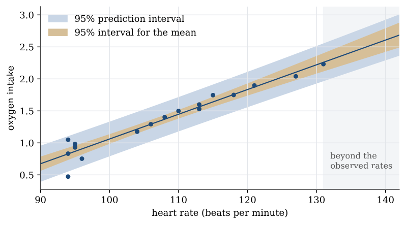
For one person, heart rate and oxygen intake are measured together 19 times.

Heart rate	94	96	95	95	94	95	94	104	104	106
Oxygen	0.473	0.753	0.929	0.939	0.832	0.983	1.049	1.178	1.176	1.292

Heart rate	108	110	113	113	118	115	121	127	131
Oxygen	1.403	1.499	1.529	1.599	1.749	1.746	1.897	2.040	2.231

Question. Fit the regression of oxygen intake on heart rate, give a 95% interval for the slope, and test whether the slope is zero.

Solution. Here \overline x=107.0 and S_{xx}=2518. The fitted line is y=-2.804+0.03865\,x. The residual standard deviation is S=0.1205, so S_1=0.1205/\sqrt{2518}=0.00240 and S_0=0.258. With t_{17;0.975}=2.110, the 95% interval for the slope is

0.03865\pm2.110\times0.00240=(0.0336,\ 0.0437).

It excludes zero. Equivalently, t=0.03865/0.00240=16.1, far beyond 2.110, so H_0:\beta_1=0 is rejected. Each extra beat per minute goes with about 0.039 more units of oxygen.

Predicting a student’s height

Worked example from Regression examples

Question. For a student with shoe size 30 cm, give a 95% interval for the mean height of such students, and a 95% interval for the height of one such student.

Solution.

predict(model1, data.frame(shoe = 30), interval = "confidence")
#        fit      lwr      upr
#   175.9217 173.4261 178.4172
predict(model1, data.frame(shoe = 30), interval = "prediction")
#        fit      lwr      upr
#   175.9217 157.2999 194.5434

The point prediction is 145.78+1.0048\times30=175.9 cm in both cases. The mean height of students with this shoe size is pinned down to within about 2.5 cm. A single student’s height is not: the prediction interval is (157.3,\ 194.5), about 37 cm wide, because a new student varies about the line with standard deviation near 9.3 cm whatever the sample size. The two intervals are the interval for the mean response and the prediction interval.

Where is the prediction interval narrowest?

Question page: Where is the prediction interval narrowest?

In simple linear regression, at which value of x is the prediction interval for a new response narrowest, and what is its half-width there? Does it shrink to zero as n\to\infty?

Worked answer (click to show)

The half-width is t_{n-2;1-\alpha/2}\,S\sqrt{1+1/n+(x-\overline x)^2/S_{xx}}, which is smallest when (x-\overline x)^2=0, at x=\overline x. There it is t_{n-2;1-\alpha/2}\,S\sqrt{1+1/n}.

As n\to\infty, t_{n-2;1-\alpha/2}\to z_{1-\alpha/2}, S\to\sigma and 1/n\to0, so the half-width tends to z_{1-\alpha/2}\,\sigma, not to zero. However much data there is, a single new response still varies about the line with standard deviation \sigma.

Used in

Taught in Linear regression, where the derivation and examples are.
Also used in Regression examples
Questions that use it (2) — Where is the prediction interval narrowest? · Rain, food, and orange yield
All 5 questions on Linear regression